2D Ising Model - Third year CMP experiment

by Bjorn Gugu; Experiment conducted from 19/01/2015 - 30/01/2015

Abstract

This report discusses a computational approach to the calculation of the heat capacity of the ferromagnetic phase transition in a 2D Ising Model. A Monte Carlo simulation was performed to calculate the average spin and magnetisation of various periodic lattices over temperature. The heat capacities were obtained and the critical temperature of the phase transition was found in relation to the lattice size. The answer of this simulation, $T_{C} = 2.267 K$ shows strong agreement with the literature value of 2.269K^[1].

Methods

All code used in this experiment was written in Python. References values were provided by an external simulation written in C++. The simulation is based on a Monte Carlo algorithm for importance sampling of thermodynamic states.

Discussion

The Ising Model

Show that the lowest possible energy for the Ising model is $E = - D N J$ , where D is the number of dimensions and N is the total number of spins. What is the multiplicity of this state? Calculate its entropy.

The total energy of a system of D dimensions and N atoms is given by $- \frac{J}{2} \sum_{i}^{N} \sum_{j \in a d j} s_{i} s_{j}$ , where J is the strength of an individual interaction. The lowest energy state is expected to be the one in which all spins are parallel. Therefore, $s_{i} s_{j} = 1$ for all interactions. A linear system assigns two direct neighbours to each atom. As the dimensions are independent of one another, every degree of freedom adds another 2 neighbours to each atom. Therefore, the amount of direct neighbours of each atom is $2 D$ and $\sum_{j \in a d j} s_{i} s_{j} = 2 D$ . This is the number of interactions per atom. In order to evaluate the total interactions, simply the sum overall atoms must be taken. The atomic interactions are constant, as previously established, therefore $\sum_{i}^{N} \sum_{j \in a d j} s_{i} s_{j} = 2 N D$ and $E = - N J D$ .

There is only one possible arrangement of spins that yields this configuration, so the number of microstates is 1. The entropy of such a system is given by $S = K_{B} l n W$ , where $K_{B}$ is Boltzmann's constant and W the number of microstates. Given that $W = 1$ , $S = 0$ .

Imagine that the system is in the lowest energy configuration. To move to a different state, one of the spins must spontaneously change direction ("flip"). What is the change in energy if this happens (D=3, N=1000)? How much entropy does the system gain by doing so?

If one atom flips spin, according to the calculation from Task 1, an atom interacts with 2D other atoms (after accounting for double-counting of interactions). The energy of each interaction is +J. The total energy however changes by 2J per interaction, as the new interaction is not only positive, but also removes a former negative interaction. The total change in energy is then 2DJ. For a system (N = 1000, D = 3) this change amounts to 6J. The number of microstates is N, as each atom is equally likely to flip. The change in entropy is therefore $S_{1} - S_{0} = K_{B} l n N - 0 = K_{B} l n N = 9.540 * 1 0^{- 23}$ .

Calculate the magnetisation of the 1D and 2D lattices in figure 1. What magnetisation would you expect to observe for an Ising lattice with D=3, N=1000 at absolute zero?

The total magnetisation of a system is given by $M = \sum_{i}^{N} s_{i}$ . For the three example systems indicated, the total magnetisations are M₁ and M₂, respectively. $M_{1} = M_{2} = 1$ , as one more up-spin entity is present than down-spin entities. For a system (D = 3, N = 1000, T = 0K) all spins are expected to align in parallel and the total magnetisation is simply the sum of all atoms: $| M | = 1000$

Calculating the energy and magnetisation

Complete the functions energy() and magnetisation(), which should return the energy of the lattice and the total magnetisation, respectively. In the energy() function you may assume that J=1.0 at all times (in fact, we are working in reduced units in which $J = k_{B}$ , but there will be more information about this in later sections). Do not worry about the efficiency of the code at the moment — we will address the speed in a later part of the experiment.

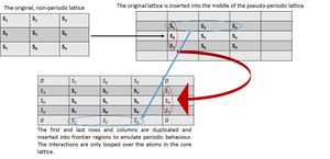
In order to calculate the energy of the system, the above equation has to be implemented into code. This can be done by looping over all atoms, calculating the interactions each atom exhibits with its neighbours. Additionally, the periodicity of the lattice has to be accounted for. While the randomly defined lattice in the initialisation of the IsingLattice class is two-dimensional, no direct connection between atoms on the "borders" of the lattice are given. Therefore a new property "periodic_lattice" was defined, which is an ndarray of size(n_rows+2, n_cols+2). The core section of this ndarray is the lattice defined as before, but the first and last rows and columns are copied from the respective lines in the original lattice (Figure 1). This pseudo-periodic lattice allows looping over all interactions of the atoms in the core section without the necessity of introducing exception clauses. The magnetisation of the lattice can simply be found by adding the values of each matrix entry, looping over both dimensions.

Run the ILcheck.py script from the IPython Qt console using the command

The values calculated by the above functions were compared to a number of previously calculated systems. It can be seen that the functions above provide exactly correct results (Figure 2).

Introduction to Monte Monte Carlo simulations

How many configurations are available to a system with 100 spins? To evaluate these expressions, we have to calculate the energy and magnetisation for each of these configurations, then perform the sum. Let's be very, very, generous, and say that we can analyse $1 \times 1 0^{9}$ configurations per second with our computer. How long will it take to evaluate a single value of $< M >_{T}$ ?

The number of energy states given for a system of N particles with n available states is given by $W = n^{N}$ . In this system, n=2, N=100, therefore $W = 2^{100}$ ≈ $1.27 * 1 0^{30}$ . Estimating an evaluation of $1 0^{9}$ states per second, a calculation of all microstates of the above systems would take approximately 10²¹ seconds - roughly 10¹⁴ years.

Implement a single cycle of the above algorithm in the montecarlocycle(T) function. This function should return the energy of your lattice and the magnetisation at the end of the cycle. You may assume that the energy returned by your energy() function is in units of $k_{B}$ ! Complete the statistics() function. This should return the following quantities whenever it is called: $< E >$ , $< E^{2} >$ , $< M >$ , $< M^{2} >$ , and the number of Monte Carlo steps that have elapsed.

An implementation of a Monte Carlo simulation essentially requires a method of comparing the probabilities of occurrence of two experimental outcomes. In this case, the ensemble average of the energy and the magnetisation of a system will be calculated. To assess the occurrence of a fluctuation in the system, a random spin flip of one spin, the energy of the lattice before and after the flip is calculated with the energy() function. The flip itself can simply be simulated by changing the sign of the given lattice entry. The algorithm for the acceptance and rejection of states was implemented via two nested if-structures. If a state is accepted, it is added to the list of accepted states, from which the average properties will be calculated via the statistics() function. The exponential factor is not explicitly entered into the average calculation, as it is already implemented in the acceptance-rejection algorithm. Instead of simply adding the newly calculated energies to a running average, lists for all four properties were calculated to be able to relate temperatures to each data point retrospectively.

The statistics() function computes the averages of the four properties energy, energy squared, magnetisation and magnetisation squared from the states stored by the montecarlostep(T) function. The entries in the respective lists are read, summed and divided by the number of Monte Carlo cycles.

If $T < T_{C}$ , do you expect a spontaneous magnetisation (i.e. do you expect $< M > \neq 0$ )? When the state of the simulation appears to stop changing (when you have reached an equilibrium state), use the controls to export the output to PNG and attach this to your report. You should also include the output from your statistics() function.

The Curie temperature T_C is the temperature at which entropic contributions balance the energetic stability of well ordered systems. Therefore, at temperatures lower than T_C, entropy cannot outweigh the energetic preference for well ordered systems. Therefore, the alignment of spins will be non-random and <M> will be non-zero. At T=0K only the lowest energy state would be occupied. At temperatures higher than absolute zero intermediate states between perfect uniform alignment and completely random alignment may be found. These manifest in the formation of regions of uniform spin that show only few disclinations. The formation of such intermediate states depends heavily on the (randomly chosen) starting conditions.

The ILanim.py function runs the simulation at T=1.0K. The system reaches the predicted equilibrium state of energy/spin = -2 and magnetisation/spin = +1 after approximately 600 Monte Carlo cycles. This corresponds to a fully aligned system. The equilibrium proves very stable, little fluctuation scan be observed (Figure 3). This is due to the low temperature at which this simulation was conducted. It is assumed that higher temperatures lead to stronger fluctuations. The average energy, energy squared, magnetisation and magnetisation squared of this system are, according statistics() function: -1.728, 3.214, -0.8476 & 0.7873.

Due to changes in the code of the statistics() function at later points in this experiment, correct averages, which span the whole range of Monte Carlo cycles, are only found with the file IsingLattice_slow.py.

Accelerating the code

Use the script ILtimetrial.py to record how long your current version of IsingLattice.py takes to perform 2000 Monte Carlo steps. This will vary, depending on what else the computer happens to be doing, so perform repeats and report the error in your average!

The ILtimetrial.py function assesses the performance of the montecarlostep(T) function. The time trial was performed 10 times on an otherwise superficially idle computer (no other programs operated by user), yielding an average computational time of 148s (rms 0.7s). Considering that over 100000 Monte Carlo steps will be calculated for multiple lattices this calculation speed is not feasible.

Look at the documentation for the NumPy sum function. You should be able to modify your magnetisation() function so that it uses this to evaluate M. The energy is a little trickier. Familiarise yourself with the NumPy roll and multiply functions, and use these to replace your energy double loop (you will need to call roll and multiply twice!).

Simply using the numpy.sum function instead of two nested for-loops allows for a faster calculation of the magnetisation of the system. The calculation of the energy however is more involved. The numpy function multiply allows the multiplication of each element in an array with its counterpart in another array. By using the roll function, each entry in the lattice array can be shifted by 1 column or row in either direction, representing both an interaction with a neighbouring element as well as implementing periodic boundary conditions. The total energy can be calculated by $- \frac{J}{2} \sum_{i}^{N} \sum_{j \in a d j} s_{i} s_{j}$ , where the inner sum $\sum_{j \in a d j} s_{i} s_{j}$ represents the interactions each atom shows with its neighbours. By creating a matrix in which each element represents the sum of the interactions of each entry's counterpart in the real lattice, this inner sum is validly expressed. The outer sum is then simply the sum over all elements of this auxiliary matrix.

Use the script ILtimetrial.py to record how long your new version of IsingLattice.py takes to perform 2000 Monte Carlo steps. This will vary, depending on what else the computer happens to be doing, so perform repeats and report the error in your average!

The updated code exhibits an average computational time of 0.616s, which is about 240 times faster than the original code. The rms was lowered to 0.00939, which is orders of magnitude lower than the average value, indicating a valid experiment.

The effect of temperature

The script ILfinalframe.py runs for a given number of cycles at a given temperature, then plots a depiction of the final lattice state as well as graphs of the energy and magnetisation as a function of cycle number. This is much quicker than animating every frame! Experiment with different temperature and lattice sizes. How many cycles are typically needed for the system to go from its random starting position to the equilibrium state? Modify your statistics() and montecarlostep() functions so that the first N cycles of the simulation are ignored when calculating the averages. You should state in your report what period you chose to ignore, and include graphs from ILfinalframe.py to illustrate your motivation in choosing this figure.

Empirically it can be seen that the time needed to achieve equilibration is less than 100 times the amount of spins in the system (Figure 4). The temperature does not seem to affect the time needed to achieve equilibrium, but the added noise creates a need for longer averaging periods (Figure 5). Considering this, the statistics() function now calculates the averages only from data points starting after n_cols*n_rows*100 steps. This interval admits a confidence interval should a different set of initial conditions demand a longer equilibration period. Additionally, the function now resets the entries of all four properties and the counter of Monte Carlo steps to enable the correct calculation of averages in future calculations.

Use ILtemperaturerange.py to plot the average energy and magnetisation for each temperature, with error bars, for an 8x8 lattice. Use your initution and results from the script ILfinalframe.py to estimate how many cycles each simulation should be. The temperature range 0.25 to 5.0 is sufficient. Use as many temperature points as you feel necessary to illustrate the trend, but do not use a temperature spacing larger than 0.5. T NumPy function savetxt() stores your array of output data on disk — you will need it later. Save the file as 8x8.dat so that you know which lattice size it came from.

As argued in task 1, the number of cycles needed to reach equilibration is N*100, where N is the number of spins in the system. This allows a fast computation (within minutes) while maintaining a high confidence interval. The variation of the critical temperature is given by the expression $T_{C, L} = \frac{A}{L} + T_{C, \inf}$ . A simple plot of $T_{C, L}$ vs. 1/L reveals that the predicted critical temperature variation will vary between 2 - 3 K. Therefore, 0.1K was chosen as an appropriate temperature step size. The total number of cycles was chosen in such a way that at least twice the amount of redundant cycles was calculated to allow for sufficient averaging steps once equilibration is achieved. The script ILplotaverage.py reads the values generated by ILtemperaturerange.py and plots the average of energy and magnetisation per spin over three data sets against temperature (Figure 6). The errorbars indicate the standard deviation.

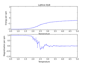
The energy per spin rises from the energy of the minimum configuration (-2) to a value closely below zero. The magnetisation starts from an initial value of +2 (perfectly ordered lattice below T_C) and falls to 0 (disordered lattice over T_C). In the steep transition between the initial and final value, great noise is observed, which is typical of a critical region. The phase transition exhibits strong over- and undershooting and generally chaotic behaviour.

The effect of system size

Repeat the final task of the previous section for the following lattice sizes: 2x2, 4x4, 8x8, 16x16, 32x32. Make sure that you name each data file that you produce after the corresponding lattice size! Write a Python script to make a plot showing the energy per spin versus temperature for each of your lattice sizes. Hint: the NumPy loadtxt function is the reverse of the savetxt function, and can be used to read your previously saved files into the script. Repeat this for the magnetisation. As before, use the plot controls to save your a PNG image of your plot and attach this to the report. How big a lattice do you think is big enough to capture the long range fluctuations?

For each lattice size three simulations were conducted to allow for fluctuations introduced by varying initial conditions. The scripts ILplot_average2.py & ILplot_average3.py' read three data sets generated for each lattice size, averages their values and calculates the energy/ magnetisation per spin. The data for all lattice sizes are plotted on the same graph (Figure 7). Error bars were omitted for legibility.

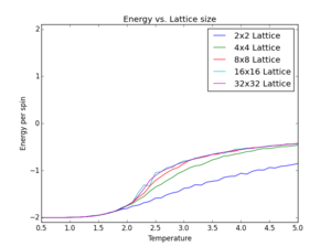
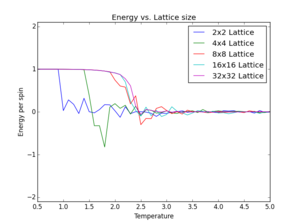
The plots produced show similar features across all lattice sizes: As seen before, the energy rises from the minimum of -2 per spin to a maximum value close to zero. The final value is proportional to the system size. Considering the plot of energy/spin vs. temperature it can be seen that the curves converge against a final value with increasing lattice size. While lattices of sizes 2x2 and 4x4 show significant deviation from this final value. Lattices of sizes 8x8 or bigger exhibit the right energetic properties and therefore capture long-range fluctuations.

Determining the heat capacity

Write a Python script to make a plot showing the heat capacity versus temperature for each of your lattice sizes from the previous section. You may need to do some research to recall the connection between the variance of a variable, Var[X], the mean of its square $< X^{2} >$ , and its squared mean $< X >^{2}$ . You may find that the data around the peak is very noisy — this is normal, and is a result of being in the critical region. As before, use the plot controls to save your a PNG image of your plot and attach this to the report.

The heat capacity of the system is given by:

$C = \frac{V a r (E)}{K_{B} T^{2}} = \frac{< E^{2} > - < E >^{2}}{K_{B} T^{2}}$

In order to calculate the heat capacity, values for the energy and energy squared vs. temperature are read from files generated beforehand (ILheatcapacity.py). As three data sets are present, averages are calculated. The Boltzmann constant can be omitted from the calculation as the energies are set in reduced units. The plots of heat capacity vs. temperature show curves with a well defined maximum (Figure 9). The maximum increases in value at higher temperatures and also shift to slightly lower temperatures. Due to the noise present at the critical region, the fit will need to be prepared from data of higher resolution. It can also be seen that the function onset is different from the final value, which is typical for a second order phase transitions, such as the one present.

Figure 9: The variation of heat capacity with temperature for various lattice sizes.

Locating the Curie Temperature

A C++ program has been used to run some much longer simulations than would be possible on the college computers in Python. You can view its source code here if you are interested. Each file contains six columns: T,E,E^{2},M,M^{2},C (the final five quantities are per spin), and you can read them with the NumPy loadtxt function as before. For each lattice size, plot the C++ data against your data. For one lattice size, save a PNG of this comparison and add it to your report — add a legend to the graph to label which is which. To do this, you will need to pass the label="..." keyword to the plot function, then call the legend() function of the axis object.

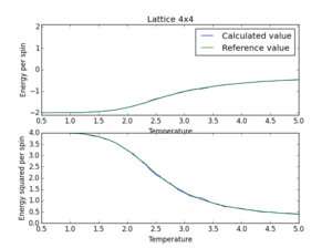
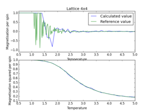
The script ILreference.py plots reference values together with the simulated values calculated above on the same graph for comparison (Figure 10, 11, 12). Attention should be paid to the different amount of data points in the two curves, which were accounted for by two different sets of temperature values. It is evident that the calculated data correlate highly with the reference data. The strongest deviations can be found in the region of the phase transition, but large fluctuations are expected in this region. The accuracy of the values could be adjusted by increasing the number of redundant steps in the Monte Carlo simulation as well as the number of averaging steps.

Write a script to read the data from a particular file, and plot C vs T, as well as a fitted polynomial. Try changing the degree of the polynomial to improve the fit — in general, it might be difficult to get a good fit! Attach a PNG of an example fit to your report.

The script ILfit1.py plots both the heat capacity as well as a polynomial fit against temperature. The degree of the fit can be chosen by the user. A range of fit degrees were tested. However, even a polynomial of degree 30 could not provide a satisfactory fit (Figure 13).

Modify your script from the previous section. You should still plot the whole temperature range, but fit the polynomial only to the peak of the heat capacity! You should find it easier to get a good fit when restricted to this region.

ILfit_updated.py reduces the range of temperatures over which the polynomial proposed in ILfit1.py is fitted. As it is of highest importance to accurately sample the region around the maximum in heat capacity, the fitting range was set to start at half the value of the maximum and end after the function has passed through half the maximum value once more - for different functional forms of heat capacity this would need to be adjusted to a more general algorithm. This value can be adjusted to different ranges to provide optimal fits. A fourth degree fit was found to be satisfactory (Figure 14).

Find the temperature at which the maximum in C occurs for each datafile that you were given. Make a text file containing two colums: the lattice side length (2,4,8, etc.), and the temperature at which C is a maximum. This is your estimate of T_{C} for that side length. Make a plot that uses the scaling relation given above to determine $T_{C, \infty}$ . By doing a little research online, you should be able to find the theoretical exact Curie temperature for the infinite 2D Ising lattice. How does your value compare to this? Are you surprised by how good/bad the agreement is? Attach a PNG of this final graph to your report, and discuss briefly what you think the major sources of error are in your estimate.

By finding the maximum in the fitted curve, the maximum in heat capacity and the critical temperature at which it occurs can be approximated. The script mentioned above writes the critical temperature at every lattice size to the output file Heatcapacity_maxima.txt. According to the relation

$T_{C, L} = \frac{A}{L} + T_{C, \infty}$

the critical temperature of an infinite 2D Ising Lattice can be extrapolated from a plot of T_{C, L} vs. $\frac{1}{L}$ . The constant A can be obtained from the gradient of the linear fit, whereas the intercept with the y-axis equals the critical temperature of an infinite lattice (Figure 15). Even though the function shows a poor correlation with a linear fit, the obtained value of $T_{C, \infty} = 2.267 K$ is very close to the literature values of 2.269K^[1] and 2.534K^[2]. The quality of the result is surprising, considering the small computational effort put into this calculation.

NJ: It's not Kelvin, it's reduced units.

Clearly any values calculated by a Monte Carlo method need both high confidence intervals (the number of redundant steps admitted before equilibration takes place) and a high number of averaging steps once equilibration is achieved. Especially the region of phase transition shows large deviations from reference values due to its chaotic nature. Secondly, the finite resolution of temperature steps creates the need for a compromise between accuracy and speed and may influence the accuracy of the result if the resolution is too little. Thirdly, the polynomial fit imposed onto simulated data introduces a negligible error.

In order to allow for the calculation of real, non-ideal properties of 2D systems, non-ideal structural properties of crystals will need to be taken into account. Additionally to the material dependent values of A and J, real crystals will show disclinations, impurities and other non-ideal properties. Due to the random distribution of such properties and their relatively low occurence, the required system size for such calculations will grow.

References

↑ ^1.0 ^1.1 Preis, Tobias, et al. "GPU accelerated Monte Carlo simulation of the 2D and 3D Ising model." Journal of Computational Physics 228.12 (2009): 4468-4477.
↑ Onsager, Lars. "Crystal statistics. I. A two-dimensional model with an order-disorder transition." Physical Review 65.3-4 (1944): 117.

[lit_value1-1] 1.0 ^1.1 Preis, Tobias, et al. "GPU accelerated Monte Carlo simulation of the 2D and 3D Ising model." Journal of Computational Physics 228.12 (2009): 4468-4477.

[lit_value2-2] Onsager, Lars. "Crystal statistics. I. A two-dimensional model with an order-disorder transition." Physical Review 65.3-4 (1944): 117.

[1]

[2]