
Rep:Mod:am4010
Inorganic Computational Laboratory
Week 1
The aim of the first week of this experiment was to become familiar with the Gaussian software (GaussView 5.0). Gaussian allows us to predict many different experimental values of a molecule, for example molecular geometry, bond lengths, bond angles, IR spectrum and also NMR spectrum. Therefore being able to manipulate molecules in Gaussian instead of measuring them in a laboratory can be extremely useful, especially when the molecular system under observation is unstable or toxic. The calculations performed in this week provided a platform for further use of the Gaussian program and revealed some insights into some Group 13 compounds of the periodic table.
BH3 Optimisation
For the first part of this module Borane was created in Gaussian and using its functions it was optimised (the nuclei were put in their lowest energy configuration according to the electronic structure of the entire molecule). The following parameters, though rather primitive, were used for this calculation and the following results obtained:
| Function | Value |
|---|---|
| File type | .log |
| Calculation type | FOPT |
| Method | B3LYP |
| Basis set | 3-21G |
| E(RB3LYP) | -26.46226349 a.u |
| Gradient | 0.0001559 a.u |
| Dipole moment | 0.00D |
| Point group | C2v |
| Time taken | 8 seconds |
| H-B-H optimised bond angle | 120.2O |
| B-H optimised bond length | 1.19Å |
The link to the calculation can be found here: File:AM BORANE OPTIMISATION.LOG
In this calculation only a 3-21G basis set was used, so although the calculation was very quick, it is clear that it also wasn't very accurate. This can be seen by the fact that it claims that BH3 has a point group of C2v is clearly incorrect. As the optimisation is carried out the nuclei are moved closer together and further apart, and the Schrodinger equation is solved for each distance between the atoms. When the lowest energy configuration is found, the atoms are said to have "converged" to this lowest energetic point. The easiest way of representing this is by using a Morse potential:

Although the example here is for a diatomic, the same principles hold for any molecule. As the atoms are moved far away there is no electronic interaction and so the potential energy converges to 0, whereas as the atoms are pushed too close together the energy increase exponentially due to energetically unfavourable nuclei-nuclei interactions. At equilibrium the potential energy is at its lowest and this represents the bond length, and it is this which Gaussian is calculating during the optimisation. Although it is important to note that this structure in some cases is only found in the gas phase, as in the solid phase other interactions may override this potential energy and cause a perturbation in the molecular geometry.
The output file given to us by Gaussian is merely a representation of which orientation of atoms will give us the lowest energy configuration of the molecule. It is important to remember that the bonds in the molecule are there for convenience, and the "true" electron configuration of the molecule does not restrict electrons between atoms, but on the contrary the Molecular Orbitals (MO's) are often delocalsied over the ENTIRE molecule. In calculating MO's later we will be able to see that Gaussian is also able to give us a picture of the "true" bonding of a molecule by providing us with the MO's. The output file also gives us a RMS gradient, which tells us if we move our atoms slightly, how much the potential energy will change by. If this energy is not sufficiently low (<0.001) then the optimisation is not complete.
Using our output file we can also check that our molecule has successfully converged to its lowest energy configuration. This can be done by clicking "Results" and then "View File". We are then given the summary that can be seen below:
 Item               Value     Threshold  Converged?
 Maximum Force            0.000323     0.000450     YES
 RMS     Force            0.000153     0.000300     YES
 Maximum Displacement     0.001140     0.001800     YES
 RMS     Displacement     0.000920     0.001200     YES
 ----------------------------
                           !   Optimized Parameters   !
                           ! (Angstroms and Degrees)  !
 --------------------------                            --------------------------
 ! Name  Definition              Value          Derivative Info.                !
 --------------------------------------------------------------------------------
 ! R1    R(1,2)                  1.1946         -DE/DX =   -0.0001              !
 ! R2    R(1,3)                  1.1943         -DE/DX =    0.0                 !
 ! R3    R(1,4)                  1.1943         -DE/DX =    0.0                 !
 ! A1    A(2,1,3)              119.8876         -DE/DX =    0.0002              !
 ! A2    A(2,1,4)              119.8876         -DE/DX =    0.0002              !
 ! A3    A(3,1,4)              120.2247         -DE/DX =   -0.0003              !
 ! D1    D(2,1,4,3)            180.0            -DE/DX =    0.0                 !
 --------------------------------------------------------------------------------
As can be seen in the information above, the calculation says "converged" for all of the parameters (force/displacement), this confirms that the parameter has converged close enough to the actual optimised value that we are seeking. However as mentioned previously it is possible to use a more advanced basis set to improve our calculation and hence the optimisation of BH3.
In order to optimise the molecule better, it was decided to use a more advanced basis set 6-31G (d,p)
The calculation gave the following results:

| BH3_OPT_631G_DP.log | |
|---|---|
| Function | Value |
| File type | .log |
| Calculation type | FOPT |
| Method | B3LYP |
| Basis set | 6-31G (d,p) |
| E(RB3LYP) | -26.61531696 a.u |
| Gradient | 0.00052014 a.u |
| Dipole moment | 0.00D |
| Point group | C2v |
| Time taken | 11 seconds |
| H-B-H optimised bond angle | 119.9O |
| B-H optimised bond length | 1.19Å |
The link to the calculation can be found here: File:BH3 OPT 631G DP.LOG
As can be seen the data has now shifted slightly, the bond angle between H-B-H is now slightly wider. As expected for a trigonal planar molecule, the bond angle is now closer to 120o. Although, the point group is still C2v. The bond angle is now closer to the expected value for a trigonal planar molecule of 120O, which is to be expected, we also have a value of the B-H bond length which is in close agreement with the literature value of 1.19Å. [2] Again by using the results of the output file we can confirm that our calculation has converged to an potential energy minima:
          Item               Value     Threshold  Converged?
 Maximum Force            0.000157     0.000450     YES
 RMS     Force            0.000074     0.000300     YES
 Maximum Displacement     0.000576     0.001800     YES
 RMS     Displacement     0.000478     0.001200     YES
 Predicted change in Energy=-1.261607D-07
 Optimization completed.
    -- Stationary point found.
                           ----------------------------
                           !   Optimized Parameters   !
                           ! (Angstroms and Degrees)  !
 --------------------------                            --------------------------
 ! Name  Definition              Value          Derivative Info.                !
 --------------------------------------------------------------------------------
 ! R1    R(1,2)                  1.1924         -DE/DX =    0.0                 !
 ! R2    R(1,3)                  1.1923         -DE/DX =    0.0                 !
 ! R3    R(1,4)                  1.1923         -DE/DX =    0.0                 !
 ! A1    A(2,1,3)              119.9463         -DE/DX =    0.0001              !
 ! A2    A(2,1,4)              119.9463         -DE/DX =    0.0001              !
 ! A3    A(3,1,4)              120.1075         -DE/DX =   -0.0002              !
 ! D1    D(2,1,4,3)            180.0            -DE/DX =    0.0                 !
 --------------------------------------------------------------------------------
Again as can be seen this convergence has taken place successfully. The calculation has given good agreement between experimental and theoretical bond lengths and angles, and so it can be clearly seen that using Gaussian can be a powerful technique for analysis. However we will now see that this is not restricted to light atoms, but can also be extended to heavier atoms.
TlBr3 Optimisation
The next part of the module was to now create a molecule of TlBr3 in GaussView, and to now optimise this molecule, however now using a slight modification of basis sets. We will now use a basis set consisting of "pseudo potentials". The idea behind this is that as Thallium is such a large atom (X = 81) using a normal basis set such as 3LYBP would take an incredibly long time to calculate as it has to take into account all of the electrons ie. 81! However our chemical intuition tells us that only valence electrons are important to take into account when considering the bonding in a molecule. Using a pseudo potential allows us to effectively "ignore" the core electrons, thus making the calculation a lot faster, whilst still maintaining some accuracy.
First of all it is important to restrict the symmetry of our molecule to D3h, the actual point group of the compound. This is to ensure that later calculations are successful as the optimisation may well calculate an incorrect point group as before. VSEPR theory allows to easily prove that TlBr3 does in fact have D3h symmetry. [3] The basis set now used is known as "LanL2DZ", this in essence a dual basis function, using a D95V on the lighter atoms whilst using Los Alamos ECP (a psuedo potential) on the heavier atoms. This calculation gave the following results:

| Function | Value |
|---|---|
| File type | .log |
| Calculation type | FOPT |
| Method | B3LYP |
| Basis set | LANL2DZ |
| E(RB3LYP) | -91.21813024 a.u |
| Gradient | 0.00000067 a.u |
| Dipole moment | 0.00D |
| Point group | D3H |
| Time taken | 41.4 seconds |
| Br-Tl-Br optimised bond angle | 120.0 |
| B-H optimised bond length | 2.65Å |
The link to the calculation can be found here: File:AM TlBr3 NEW.log
The calculation has predicted a Br-Tl-Br bond angle of 120O, as we would expect for the trigonal planar structure, it has also calculated a Tl-Br bond length of 2.65Å, which is in good agreement with the literature value of 2.6182Å. [4] Again we check to see whether our calculation has converged:
Item               Value     Threshold  Converged?
 Maximum Force            0.000001     0.000015     YES
 RMS     Force            0.000001     0.000010     YES
 Maximum Displacement     0.000016     0.000060     YES
 RMS     Displacement     0.000011     0.000040     YES
 Predicted change in Energy=-3.389481D-11
 Optimization completed.
    -- Stationary point found.
                           ----------------------------
                           !   Optimized Parameters   !
                           ! (Angstroms and Degrees)  !
 --------------------------                            --------------------------
 ! Name  Definition              Value          Derivative Info.                !
 --------------------------------------------------------------------------------
 ! R1    R(1,2)                  2.6512         -DE/DX =    0.0                 !
 ! R2    R(1,3)                  2.6512         -DE/DX =    0.0                 !
 ! R3    R(1,4)                  2.6512         -DE/DX =    0.0                 !
 ! A1    A(2,1,3)              120.0            -DE/DX =    0.0                 !
 ! A2    A(2,1,4)              120.0            -DE/DX =    0.0                 !
 ! A3    A(3,1,4)              120.0            -DE/DX =    0.0                 !
 ! D1    D(2,1,4,3)            180.0            -DE/DX =    0.0                 !
 --------------------------------------------------------------------------------
The calculation has indeed converged. This example shows that the power of using pseudo-potentials, the calculation was still able to maintain high levels of accuracy in bond length and angle, even though the calculation was relatively quick. These potentials will become very useful as we move onto more complex molecules with a number of heavy atoms. We can also see that the energy of TlBr3 is much lower than BH3, this is probably beacuse we know that Boron dimersises in reality to form diborane, whereas as Tl is large and is surrounded by 3 electron withdrawing Br atoms this stabilises the molecule and will allow it to exist as a monomer. Therefore when comparing the monomers BH3 will be much higher in energy as it doesnt exist in this form, where the B has only 6 electrons around itself, so it doesnt fulfill the octet rule. Tl also does not fulfill the rule, but as mentioned the Br atoms will stabilise it.
BBr3 Optimisation
The aim of this calculation was to be able to mix the pseudo potentials used in the previous example, and use a full basis set on a lighter atom at the same time. A good example of this is BBr3, where a pseudo potential can be used on the Br atoms whilst a full basis set can be used on the lighter B atom. To do this requires use of the basis set GEN, which will allow us to specify which basis set we wish to use on each atom. The job was set up as previously however instead of submitting it immediately the file was manually manipulated to give the B atom a 6-31G(d,p) full basis set whilst the Br atoms were given the LanL2DZ pseudo potential basis set. This calculation gave the following results.

| Function | Value |
|---|---|
| File type | .log |
| Calculation type | FOPT |
| Method | B3LYP |
| Basis set | GEN |
| E(RB3LYP) | -64.42903587 a.u |
| Gradient | 0.01418124 a.u |
| Dipole moment | 0.00D |
| Point group | C2v |
| Time taken | 35.8 seconds |
| Br-B-Br optimised bond angle | 119.9 |
| Br-B optimised bond length | 2.02Å |
The link to the calculation can be found here: DOI:10042/21656
The calculation was again relatively quick, and gave results which are as to be expcted for the bond angle of a trigonal planar compound, however the bond length calculation is of more interest. The literature value of this bond length is 1.893Å[5], whereas the bond length calculated is 2.02Å. This is quite a significant difference compared to earlier calculations were we have always beenw ithin 10 pm of the experimental value. What could explain such a difference? The answer lies in our use of pseudo potentials. We have assumed that the core electrons on Br have no effect on the electronic structure, of course in reality this is not the case. Whilst the impact may be small in comparison to valence electrons it is certainly noticeable and it is this assumption that causes our bond length to differ more significantly from the literature. Again we can check that the calculation was completed successfully and that this is not the source of the error.

  Item               Value     Threshold  Converged?
 Maximum Force            0.000108     0.000450     YES
 RMS     Force            0.000056     0.000300     YES
 Maximum Displacement     0.000497     0.001800     YES
 RMS     Displacement     0.000276     0.001200     YES
 Predicted change in Energy=-5.201728D-08
 Optimization completed.
    -- Stationary point found.
                           ----------------------------
                           !   Optimized Parameters   !
                           ! (Angstroms and Degrees)  !
 --------------------------                            --------------------------
 ! Name  Definition              Value          Derivative Info.                !
 --------------------------------------------------------------------------------
 ! R1    R(1,2)                  1.9338         -DE/DX =    0.0                 !
 ! R2    R(1,3)                  1.9342         -DE/DX =   -0.0001              !
 ! R3    R(1,4)                  1.9338         -DE/DX =    0.0                 !
 ! A1    A(2,1,3)              119.9809         -DE/DX =    0.0001              !
 ! A2    A(2,1,4)              120.0381         -DE/DX =   -0.0001              !
 ! A3    A(3,1,4)              119.9809         -DE/DX =    0.0001              !
 ! D1    D(2,1,4,3)            180.0            -DE/DX =    0.0                 !
 --------------------------------------------------------------------------------
As can be seen the error must come from the original parameters of the calculation as the calculation itself has converged towards the potential energy minima. This demonstrates that although Gaussian is on the whole accurate, changing the basis set of our calculation has an enormous impact of the final data that we get from the program.
Structural comparisons of BH3,TlBr3 and BBr3
The following table shows a summary of the information gathered from the calculations so far, the bond lengths of all the compunds compared to their experimental values:
| Bond | Calculated Bond Length (Å) | Exprimental Bond Length (Å) | % difference |
|---|---|---|---|
| B-H | 1.19 | 1.19000 | 0.39% |
| Tl-Br | 2.65 | 2.61820 | 3.29% |
| B-Br | 2.02 | 1.89300 | 6.29% |
The degree of accuracy clearly varies in these compounds, depending on which basis set is used as previously discussed. When comparing BH3 it is clear that the changing of the ligand from H to Br has increased the bond length by almost double, clearly there ar the sam number of electrons in each bond (both single bonds) and so the reason for the difference must lie in the nature of the ligand. Clearly as Br is a much bigger atom than H, its atomic orbitals will be more diffuse than H. This means that the distance that the B and Br need to be in order to come to the lowest energetic point is going to be larger than for H. This will therefore increase the equilibrium bond distance. Br has electron density spread out over a larger area than H and so if it were as close as H this would clearly be unfavourable as the nuclei would then start interacting, this is a negative interaction and so the potential nergy would become unfavourable. Converesly H and B are comparitively similar in size, they will have a strong orbital overlap, and so we expect to see a stronger interaction and a shorter bond, which is what we observe.
We can then compare what difference the central atom has on bond distance, as opposed to the ligand, by comparing BBr3 and TlBr3. Again bond order is not a factor in this as both molecule have bond order of 1 between the central atom and the ligand, so clearly the explaination in the difference in bond length lies in th nature of the central atom. The bond length has increased from 1.893A in B-Br to 2.6182A to Tl-Br, this difference again lies in the size of the atom. Tl is in period 6 of the periodic table whilst B is in period 2 (both elements are in group 13) and so clearly Tl is a much larger atom than B as it will have a heavier nucleus and more electron density. As with the Br and H comparison, Tl orbitals will be much more diffuse than the B and so the distance required to get an electronically favourable interaction will be much larger, simply because the central atom is much larger.
I feel it is important to note that in this bond length analysis I have used the literature values rather than the calculated values. This is because for the calculations we have used different basis sets for each one. Each basis set contains a different set of approximations when calculating the minima of the potential energy surface and so to compare them would be misleading as each basis set has used a different method for calculating the bond length.
On some output files in Gaussian it has also been observed that there are no bonds, however all the atoms do appear and in the correct shape ie. trigonal planar. Is this a mistake in the program? No! We must remember that the very nature of the chemical bond is merely a convenience, and allows us to simplify the electronic structure of our molecule. Electrons are not merely localised between atoms but are rather spread over an entire molecule, we must remember that a Molecular Orbital is just a probability density mathematical function which tells us that it is likely to find an electron in this region of space. MO diagrams allow us to visualise what happens when all of the atomic orbitals are combined (of the correct symmetry), and then we are able to construct our molecular orbitals. The nature of the MO's depends on the nature of the system under investigation.
The fact that Gaussian has ignored the bonds does not mean it is incorrect. The very nature of a "bond" is simply a region of high electron density, or where the probability of finding an electron is high. If all of the MO's of our molecules are diffuse, ie. spread out across he molecule, then it would be an unrealistic interpretation to say that the electrons are merely confined to between our central atoms and our ligands. Using 2c-2e bonds is a time-saving tool which is reliable and allows chemists to simplify the mathematics behind electron density functions so that it is much simpler for us to see the important electron density information of our molecule. For example in Borane we have 3 "single" B-H bonds, the MO diagram is likely to prove that electrons do not simply sit between atoms, however this interpretation allows us to rationalise the structure of Borane simply and effectively instead of having to draw an MO diagram. Whilst drawing this diagram is convenient for Borane, it certainly is not for larger molecules, and creating such diagrams is far from trivial.
Frequency analysis of BH3
One often used function of Gaussian is to predict the vibrational modes of a molecule, we can then use this information to predict the IR stretching frequencies of the molecule. This vibrational analysis was performed on my optimised Borane molecule as seen previously, however the calculation was now a "frequency" calculation, which gave the following results:
| Function | Value |
|---|---|
| File type | .log |
| Calculation type | FREQ |
| Method | B3LYP |
| Basis set | 6-31G (d,p) |
| E(RB3LYP) | -26.61531948 a.u |
| Gradient | 0.00041801 a.u |
| Dipole moment | 0.00D |
| Point group | D3h |
| Time taken | 15.0 seconds |
The link to the calculation can be found here: File:ADAMMUNRO BH3 FREQ.LOG
To confirm that the job has run correctly we can look at the results of the vibrational analysis:
Low frequencies ---   -1.2424   -1.0105   -0.0055    3.9820   10.9329   10.9795
 Low frequencies --- 1162.9906 1213.1788 1213.1815
As can be seen the first 6 frequencies are all close to 0cm-1, these frequencies are related to the fact that molecules have 3N-6 molecular vibrations, these 6 vibrations are related to changes of the centre of mass of the molecule, and so technically should all be 0cm-1, however the fact that they are all within ±15cm-1 of 0 is sufficient for our purposes. We can also use Gaussian to view the vibrational modes of our molecule, a summary of these vibrations for Borane is provided below:
| No. | Form of the vibration | Description | Frequency (cm-1) | Intensity | Symmetry |
|---|---|---|---|---|---|
| 1 |  |
The H atoms move in a concerted fashion in and out of the plane of the molecule whilst the B atom remains stationary | 1163 | 92 | A2' |
| 2 |  |
1 H and the B atom remain stationary, whilst the other 2 H atoms perform a scissor motion | 1213 | 14 | E' |
| 3 |  |
The B atom remains stationary, whilst 2 H atoms perform a strectching motion asymmetrically, the other H atom moves more drastically out of its equilibrium position | 1213 | 14 | E' |
| 4 |  |
The H atoms move concertedly towards and away from the B atom | 2571 | 0 | A1' |
| 5 |  |
The B and 1 H atom remain stationary, whilst the other H atoms stretch asymmetrically | 2703 | 127 | E' |
| 6 |  |
The B atom remains stationary whilst 2 H atoms perform a small symmetric stretch, whilst the other H atom performs a large asymmetric stretch | 2703.45 | 127 | E' |
Gaussian can also give us a prediction of what the IR spectrum of Borane will look like using the information from the frequency analysis calculation:

It is clear from the predicted IR spectrum that we have 3 peaks, and hence 3 vibrational modes. However the frequency calculation predicted that there would be 5 peaks (1 of the 6 peaks had an intensity of 0), how do we explain this? It can be seen that vibrations 2 & 3, and vibrations 5 & 6, have the same absorbing frequency. This is because looking at the symmetry we can see we have E symmetry, meaning that these vibrations are degenerate as they both cause exactly the same dipole when they act on the molecule, and each of the vibrational energy levels have the same energy. This means it must take the same wavelength of light to cause this vibrational transition, and so the peaks overlap in the spectrum so that all we can see is a solitary high absorbance peak. The same argument can be made for vibrations 4 & 5.
Frequency analysis of TlBr3
It was decided to also record the vibrational frequencies of TlBr3, a comparison could then be made between the BH3 which used a full 6-31G basis set due to a light molecule, versus the TlBr3 which used a pseudo potential as it is a heavy molecule. The calculation is summarised in the table below:
| Function | Value |
|---|---|
| File type | .log |
| Calculation type | FREQ |
| Method | B3LYP |
| Basis set | 6-31G (d,p) |
| E(RB3LYP) | -91.21813024 a.u |
| Gradient | 0.00000067 a.u |
| Dipole moment | 0.00D |
| Point group | D3h |
| Time taken | 22.0 seconds |
The link to the calculation can be found here: File:AM TLBR3 FREQ NEW.LOG
The frequency anaylsis gave the following low frequencies:
 Low frequencies ---   -0.0013   -0.0006    0.0000    1.8492    2.6414    2.6414
 Low frequencies ---   46.6990   46.6991   51.9486
Again we were able to use Gaussian to animate the vibrational modes that it had predicted. A summary of this information, including a description of the mode[6] on the vibrational modes is provided in the table below:
| No. | Form of the vibration | Description | Frequency (cm-1) | Intensity | Symmetry |
|---|---|---|---|---|---|
| 1 |  |
The Tl and 1 Br atom remain stationary whilst the other 2 Br atoms perform a scissor motion | 47 | 4 | E' |
| 2 |  |
The Tl atom remains stationary whilst 2 Br atoms perform a scissor motion, and the other Br atom performs a rocking motion with respect to the other 2 Br atoms | 47 | 4 | E' |
| 3 |  |
The Tl atom remins stationary while the Br atoms move concertedly out of the plane performing a twist motion | 52 | 6 | A2' |
| 4 |  |
The Tl atom remians stationary whilst the Br atoms perform a concerted symmetric stretch | 165 | 0 | A1' |
| 5 |  |
The Tl atom remains stationary, 2 Br atoms perform a symmetric stretch, whilst the other Br atom performs an asymmetric stretch with a larger displacement vector | 211 | 25 | E' |
| 6 |  |
The Tl atom remains stationary whilst 2 Br atoms perform an asymmetric stretch | 211 | 25 | E' |
As done previously, Gaussian also provides us with a prediction of the IR spectrum in the gas phase, this can be found in figure 7 below:

As we can see the two IR spectrum are very similar as to be expected due to the same molecular geometry, however a full comparison certainly would reveal some insights, as can be read in the next section.
Comparison of the vibrational frequencies of BH3 and TlBr3
| Symmetry | BH3 Stretch (cm-1) | TlBr3 Stretch (cm-1) |
|---|---|---|
| A2' | 1163 | 52 |
| E' | 1213, 1213, 2703, 2703 | 47, 47, 211, 211 |
| A1' | 2571 | 165 |
When comparing the vibrational modes and their energies of our two molecules, the first thing that we immediately see is that the energy of the vibrational modes of BH3 are much higher than TlBr3. What can we infer from such a difference? One explanation for this result is that as the Tl and Br atoms are much heavier than their early period counterparts, their orbitals will be more diffuse and so the overlap between the atomic orbitals will not be as good. As we have a weaker bond between the two atoms it will naturlly be easier to "stretch" it and so the energy for the transition will be lower. We can see this in the animations where the BH3 vibrations happen much faster than the TlBr3, simply because they are lighter.
It is also interesting to see that there has also been a re-orgainsation of the vibrational modes, whereas in BH3 the lowest energy transition was the asymmetric stretch with A1' symmetry, this mode is now higher in energy in the TlBr3 spectrum and has now got E' symmetry. Also the A1' in the TlBr3 spectum is now at a lower frequency than the E', unlike the BH3 spectrum where these vibrational modes where swapped in frequency. As stated we do have the same number of vibrations and the same type and number of symmetries, despite the modes being re-ordered. This is to be expected as the molecules have the same molecular geometry, D3h, and so we would expect the vibrations in each molecule to be similar which indeed they are. Both of the spectra have 2 peaks at a lower energy, and a further 3rd peak at a much higher energy. In the BH3 spectra however the two lower energy peaks are clearly separated whereas in the TlBr3 there is a clear overlap of these two peaks as they are closer in energy. It is expected that these modes would be close as they are only 8cm-1 apart whereas in the BH3 this is a much larger value leading to two clearly separate peaks. Another difference is that the peaks in the TlBr3 spectrum are of a much lower intensity than the BH3 spectrum, a reason for this may be that the siza of the dipole in the Tl-Br stretches is lower than in the B-H strectch, and so the intensity will be lower.
We can also see in both spectra that one of the E peaks lies much higher than the other 2 peaks. The reason for this is that the higher peaks are dominated by strong asymmetric stretches, whilst the lower energy peaks have symmetric stretches. An asymmetric stretch may take more energy to activate as it leads to a more perturbed change in dipole than the symmetric stretch. Thus we will have a more extreme change in the electron density as one bond is stretched whilst the other is compressed. The symmetric stretch leads to two bonds being stretched and compressed simultaneously and so the electron density while still undergoing a change, the change is not as dramatic and so does not require as much energy to activate.
It is important to use the same basis set in both the optimisation and the frequency analysis. The reason for this is that each basis set calculates the energies in a unique way, they are not compatible with one another. Each basis set starts from a different point on the potential energy surface, and so if we are doing a different calculation, the new basis set will start from a point on the potential energy surface that is different from the first basis set. The energy therefore will not converge to the lowest possible point and so our calculation of the energy will not be correct.
The reason for carrying out the frequency analysis is twofold. We can first see if our energy has conformed to a minimum as it should do, and also we can predict what the gas phase IR spectrum should look like. Molecules have 3N-6 vibrations, and so in the cases that we have studied thus far we would expect to see (3 x 4) - 6 = 6 vibrational modes in our molecule. The - 6 vibrations do exist however they are translational and rotational modes, not vibrational. Therefore we would expect the energies to be at 0cm-1 as they do not require vibrational energy (IR radiation) to be activated. However in our Gaussian calculation we have clearly seen that these 6 vibration are small but crucially are not 0cm-1, what can we infer from this? Well as Gaussian is using approximations to calculate its results, there will always be some deviation from ideality. The closer these vibrations are to 0cm-1 the closer we are to the real energy of the molecule, the reason some of the modes may be higher is that the calculation has not quite converged on the "true" value of the energy, and so the modes do "exist". By performing more optimisations and using higher basis sets, we are able to see these values converge towards 0cm-1, as our molecule converges towards its true minima on the potential energy surface.
The other function of the frequency analysis is that we can also use it to calculate a predicted gas phase IR spectra. We know that vibrational modes can be probed using IR radiation, and Gaussian allows to calculate the energy in wavenumbers required to activate these modes, from this information it can then construct the IR spectra. As stated we should be able to see 6 vibrations, indeed this is the case in the frequency analysis. However we can only see 3 peaks in the spectrum, due to the reasons previously discussed.
Molecular Orbitals of BH3
Another useful tool of Gaussian is that we can calculate the MO's for our BH3 molecule. In order to do this we open our optimised BH3 from earlier (this time using the checkpoint file rather than the output file), and then set the method from "Optimisation" to "Energy" and inlcude the keywords "pop=full" so that the MO analysis is activated in the clalculation. We can also turn on the NBO (natural bond orbitals) analysis.
The link to the calculation can be found here: DOI:10042/21648
Once the calculation is complete, we can use Gaussians features to visualise the MO's. In figure 8 below, I have compared the calculated MO's to a MO diagram that I have constructed myself, using a Linear Combination of Atomic Orbitals (LCAO) theory:

As we can see the calculated MO's are remarkably similar to the LCAO orbitals. The MO's are practically the same and it would be appropriate to say that the differences if any are minimal. This tells us that LCAO can be quite useful when predicting the MO of molecules as they are very similar. For more complex molecules the Gaussian calculations would clearly take longer, however we can see that the relatively simple method of LCAO can give us very accurate results from quite a simple, non time-consuming method.
A complete analysis of NH3
The next task was to undergo a complete analysis of NH3, this involved optimising the molecule and then performing a frequency analysis. Finally we also carried out a population analysis in order to determine the Molecular Orbitals. First a molecule of NH3 was created in Gaussian and optimised according to a 6-31G basis set. We can go straight to this advanced basis set as we are probing a small molecule, any bigger than this and it would be wise to first perform a lower basis set before moving on to a more advanced one. This calculation was done according to the following parameters, and yielded the following results:
| Function | Value |
|---|---|
| File type | .log |
| Calculation type | FOPT |
| Method | B3LYP |
| Basis set | 6-31G (d,p) |
| E(RB3LYP) | -56.55664136 a.u |
| Gradient | 0.00835900 a.u |
| Dipole moment | 1.64 D |
| Point group | C3v |
| Time taken | 10.0 seconds |
The link to the calculation can be found here: File:AM NH3 OPTIMISATION.LOG
Again we can confirm the optimisation has converged using the output file:
 Item               Value     Threshold  Converged?
 Maximum Force            0.000024     0.000450     YES
 RMS     Force            0.000012     0.000300     YES
 Maximum Displacement     0.000079     0.001800     YES
 RMS     Displacement     0.000053     0.001200     YES
 Predicted change in Energy=-1.629717D-09
 Optimization completed.
    -- Stationary point found.
                           ----------------------------
                           !   Optimized Parameters   !
                           ! (Angstroms and Degrees)  !
 --------------------------                            --------------------------
 ! Name  Definition              Value          Derivative Info.                !
 --------------------------------------------------------------------------------
 ! R1    R(1,2)                  1.018          -DE/DX =    0.0                 !
 ! R2    R(1,3)                  1.018          -DE/DX =    0.0                 !
 ! R3    R(1,4)                  1.018          -DE/DX =    0.0                 !
 ! A1    A(2,1,3)              105.7413         -DE/DX =    0.0                 !
 ! A2    A(2,1,4)              105.7486         -DE/DX =    0.0                 !
 ! A3    A(3,1,4)              105.7479         -DE/DX =    0.0                 !
 ! D1    D(2,1,4,3)           -111.8631         -DE/DX =    0.0                 !
As previously we can also perform the frequency analysis to confirm that we have a potential energy minima, this calculation yielded the following results:
| Function | Value |
|---|---|
| File type | .log |
| Calculation type | FREQ |
| Method | B3LYP |
| Basis set | 6-31G (d,p) |
| E(RB3LYP) | -56.55776872 a.u |
| Gradient | 0.00000328 a.u |
| Dipole moment | 1.85 D |
| Point group | C3v |
| Time taken | 13.0 seconds |
The link to this calculation can be found here: File:AM NH3 FREQUENCY.LOG
By using the low frequencies we can see if the calculation has converged to the minima:
 Low frequencies ---  -10.4043   -9.3926   -9.3923   -0.0012    0.0006    0.0087
 Low frequencies --- 1089.3370 1693.9196 1693.9196
As we can see the low frequencies are within +-15cm-1 of 0, and so we can say that this caclulation, for our purposes has converged to the true minima.
| No. | Form of the vibration | Description | Frequency (cm-1) | Intensity | Symmetry |
|---|---|---|---|---|---|
| 1 |  |
The N atom remins stationary while the H atoms move concertedly out of the plane performing a twist motion | 1089 | 145 | A1' |
| 2 |  |
The N atom remains stationary whilst 2 H atoms perform a scissor motion, and the other H atom performs a rocking motion with respect to the other 2 H atoms | 1694 | 14 | E' |
| 3 |  |
The N atom remains stationary whilst 2 H atoms perform a scissor motion, the other H atom performs a rocking motion with respect to the other 2 H atoms | 1694 | 14 | E' |
| 4 |  |
The N atom remians stationary whilst the H atoms perform a concerted symmetric stretch | 3461 | 1 | A1' |
| 5 |  |
The N atom remains stationary whilst 2 H atoms perform an asymmetric stretch | 3590 | 0 | E' |
| 6 |  |
The N atom remains stationary, 2 H atoms perform a symmetric stretch, whilst the other H atom performs an asymmetric stretch with a larger displacement vector | 3590 | 0 | E' |
The predicted gas-phase IR spectrum looks as follows:

We can see again that this spectrum is similar to the other molecules that I have already probed, at first sight we would expect this as all of the molecules have the generic formula EX3. However we can see that the molecules have different point groups and so one might expect that we would have different vibrational modes. This seems to have had little effect on our spectrum, on the contrary aside from re-ordering of modes and a difference in strectching frequency the IR spectra are practically synonymous.
A Molecular Orbital analysis was also carried out on NH3, this is very similar to the BH3 that can be seen in figure 7, the only difference in this diagram would be that the N atomic orbitals will be lower in energy beacuse N is more electronegative than B, and so our bonding Molecular Orbitals will be of a lower energy, whilst the anti-bonding Molecular Orbitals will be of higher energy than in the BH3 MO diagram.
The link to the MO calculation can be found here: File:AM NH3 MO.LOG
Another tool that Gaussian allows us to use is NBO(Natural Bond Orbital) analysis. This allows us to see the charge distribution on our molecule, and do a complete analysis on the molecular orbitals that we have calculated. On performing a charge distribution, the following image appeared:

When using this analysis, bright red signifies a very strong negative charge whilst bright green shows a strong positive charge. As expected in figure 10 we see that the N atom is negatively charged, this is to be expected as we know that N is highly electronegative. Conversely each H atom is slightly positively charged, again to be expected as the N is pulling electron density toward itself from all of the H atoms, so the overall N negative charge will be shared equally between the 3 H atoms. It is important to note that our charges cancel to 0, as of course NH3 is a neutrally charged molecule overall.
N charge: -0.717
H charge: +0.239
As can be seen, the NBO analysis allows us to gain a qualitative picture of the electron density in the molecule. Something that MO analysis alone would not be able to do. By looking at the output file we can actually gain much more information about our molecule, such as energy of the molecular orbitals, occupancy of the orbitals and also the hybridisation of the atomic orbitals. Another interesting not is that we can see from the output file if any significant MO mixing has taken place, if so we can then adapt our MO diagram as necessary, thus this can be a very powerful tool when necessary.
Calculating the association energy of NH3-BH3
We can also use Gaussian to calculate bond energies. We know that NH3 is a Lewis base, and BH3 is a Lewis Acid, and so it is entirely reasonable that these molecules would bond to form a Lewis Acid-Base adduct. We have already calculated the energies of the reactants, and so by calculating the energy of the product we can determine the N-B bond strength. Firstly we must create a molecule of H3N-BH3 in Gaussian and optimise it. This was done according to the following parameters and yielded the following results:
| Function | Value |
|---|---|
| File type | .log |
| Calculation type | FOPT |
| Method | B3LYP |
| Basis set | 6-31G (d,p) |
| E(RB3LYP) | -83.22415206 a.u |
| Gradient | 0.00335131 a.u |
| Dipole moment | 5.51 D |
| Point group | C1 |
| Time taken | 1 minutes 47 seconds |
The calculation was checked to see if it had reached a potential energy minima:
 Item               Value     Threshold  Converged?
 Maximum Force            0.000137     0.000450     YES
 RMS     Force            0.000038     0.000300     YES
 Maximum Displacement     0.001015     0.001800     YES
 RMS     Displacement     0.000223     0.001200     YES
 Predicted change in Energy=-1.131131D-07
 Optimization completed.
    -- Stationary point found.
                           ----------------------------
                           !   Optimized Parameters   !
                           ! (Angstroms and Degrees)  !
 --------------------------                            --------------------------
 ! Name  Definition              Value          Derivative Info.                !
 --------------------------------------------------------------------------------
 ! R1    R(1,8)                  1.2097         -DE/DX =    0.0                 !
 ! R2    R(2,8)                  1.2097         -DE/DX =    0.0                 !
 ! R3    R(3,8)                  1.2097         -DE/DX =    0.0                 !
 ! R4    R(4,7)                  1.0185         -DE/DX =    0.0                 !
 ! R5    R(5,7)                  1.0185         -DE/DX =    0.0                 !
 ! R6    R(6,7)                  1.0185         -DE/DX =    0.0                 !
 ! R7    R(7,8)                  1.6686         -DE/DX =   -0.0001              !
 ! A1    A(4,7,5)              107.861          -DE/DX =    0.0                 !
 ! A2    A(4,7,6)              107.861          -DE/DX =    0.0                 !
 ! A3    A(4,7,8)              111.0371         -DE/DX =    0.0                 !
 ! A4    A(5,7,6)              107.8608         -DE/DX =    0.0                 !
 ! A5    A(5,7,8)              111.0372         -DE/DX =    0.0                 !
 ! A6    A(6,7,8)              111.0371         -DE/DX =    0.0                 !
 ! A7    A(1,8,2)              113.9009         -DE/DX =    0.0                 !
 ! A8    A(1,8,3)              113.9009         -DE/DX =    0.0                 !
 ! A9    A(1,8,7)              104.5637         -DE/DX =    0.0001              !
 ! A10   A(2,8,3)              113.9006         -DE/DX =    0.0                 !
 ! A11   A(2,8,7)              104.5636         -DE/DX =    0.0001              !
 ! A12   A(3,8,7)              104.5638         -DE/DX =    0.0001              !
 ! D1    D(4,7,8,1)            180.0013         -DE/DX =    0.0                 !
 ! D2    D(4,7,8,2)            -59.9986         -DE/DX =    0.0                 !
 ! D3    D(4,7,8,3)             60.0012         -DE/DX =    0.0                 !
 ! D4    D(5,7,8,1)            -59.9986         -DE/DX =    0.0                 !
 ! D5    D(5,7,8,2)             60.0015         -DE/DX =    0.0                 !
 ! D6    D(5,7,8,3)            180.0012         -DE/DX =    0.0                 !
 ! D7    D(6,7,8,1)             60.0012         -DE/DX =    0.0                 !
 ! D8    D(6,7,8,2)            180.0013         -DE/DX =    0.0                 !
 ! D9    D(6,7,8,3)            -59.9989         -DE/DX =    0.0                 !
 --------------------------------------------------------------------------------
As we can see this is the case. The link to the file can be found here: DOI:10042/21691
A frequency analysis was then carried out to confirm this minima:
| Function | Value |
|---|---|
| File type | .log |
| Calculation type | FREQ |
| Method | B3LYP |
| Basis set | 6-31G (d,p) |
| E(RB3LYP) | -83.22415207 a.u |
| Gradient | 0.00335128 a.u |
| Dipole moment | 5.5120 D |
| Point group | C1 |
| Time taken | 2 minutes 3.7 seconds |
The link to this calculation can be found here:DOI:10042/21693
As can be seen in the data below we have very low "low" frequencies which are close to 0cm-1, so we can assume this is a true minima:
Low frequencies ---   -2.9959   -2.4534   -0.0015   -0.0012   -0.0011    1.0933
 Low frequencies ---  263.4287  632.9863  638.4438
As there are 18 vibrational modes for this molecule, I feel it inappropriate to display them all, however the output file does tell us that all of the intensities are greater than 0.00, which again leads us to the assumption that this is a true minima. This is summarised below:
| Frequency (cm-1) | Intensity | Frequency (cm-1) | Intensity | Frequency (cm-1) | Intensity |
|---|---|---|---|---|---|
| 263 | 0 | 633 | 14. | 638 | 4 |
| 639 | 4 | 1069 | 41 | 1069 | 41 |
| 1196 | 109 | 1204 | 3 | 1204 | 3 |
| 1329 | 114 | 1676 | 28 | 1676 | 28 |
| 2472 | 67 | 2532 | 231 | 2532 | 231 |
| 3464 | 3 | 3581 | 28 | 3581 | 28 |
Now that we have optimised our adduct, we can now compar the energies of the reactants and products, this information is summarised in the table below:
| Molecule | E(B3LYP)(a.u) |
|---|---|
| H3N-BH3 | -83.22415207 |
| NH3 | -56.55776872 |
| BH3 | -26.61531948 |
Therefore the difference in energy ΔE = (-83.22415207) - (-56.55776872 + -26.61531948 ) = -0.05106387 a.u.
This converts to an association energy of ~ -134.09 kJ mol-1 and so from this we can conclude that the B-N bond strength is +134.09 kJ mol-1. The literature value for the B-N bond strength is +377.9 kJ mol-1[7], as we can see this a rather large increase on our calculated value. The reason for this is probably due to the fact that Gaussian makes many assumptions in its calculations using the basis sets we have employed, to get a value for the bond strength which is more consistent with the experimental value would require use of a more powerful basis set, and would require a lot more time.
Week 2
During the 2nd week of the laboratory a study of aromaticity was undertaken in benzene and its isoelectronic species containing N and B. The properties of Borazine were also investigated. All of these molecules are 6 membered rings and so it was interesting to see how the energy and Molecular Orbitals of the molecules changed as we moved from a hydrocarbin cyclic system to a heterocyclic charged system. Using the techniques practiced in the first week we were able to gain a qualitative picture of the structure, energy and bonding in these compunds, and then use the information from the output files of Gaussian to perform a comparison of the systems in terms of their energy and bonding.
Analysis of C6H6
Firstly an optimisation of Benzene must be carried out. As Gaussian provides a "benzene" fragment which is already in a planar geometry, it is reasonable to assume that we can use a advanced 6-31g basis set immediately (as opposed to optimising with a 3-21g and then moving up) as the molecule is already in its preferred conformation. Therefore for the optimisation it was decided to use a 6-31g (d,p) basis set, which yielded the following results:
| Function | Value |
|---|---|
| File type | .log |
| Calculation type | FOPT |
| Method | B3LYP |
| Basis set | 6-31G (d,p) |
| E(RB3LYP) | -232.25820319 a.u |
| Gradient | 0.00000196 a.u |
| Dipole moment | 0.00 D |
| Point group | C1 |
| Time taken | 3 minutes 35 seconds |
The link to the file can be found here: File:BENZENE OPT1.LOG
In order to confirm we have minimum energy we again check the Output file and the convergence data:
 Item               Value     Threshold  Converged?
 Maximum Force            0.000013     0.000015     YES
 RMS     Force            0.000004     0.000010     YES
 Maximum Displacement     0.000054     0.000060     YES
 RMS     Displacement     0.000017     0.000040     YES
 Predicted change in Energy=-1.959731D-09
 Optimization completed.
    -- Stationary point found.
                           ----------------------------
                           !   Optimized Parameters   !
                           ! (Angstroms and Degrees)  !
 --------------------------                            --------------------------
 ! Name  Definition              Value          Derivative Info.                !
 --------------------------------------------------------------------------------
 ! R1    R(1,2)                  1.3964         -DE/DX =    0.0                 !
 ! R2    R(1,6)                  1.3963         -DE/DX =    0.0                 !
 ! R3    R(1,7)                  1.0863         -DE/DX =    0.0                 !
 ! R4    R(2,3)                  1.3963         -DE/DX =    0.0                 !
 ! R5    R(2,8)                  1.0863         -DE/DX =    0.0                 !
 ! R6    R(3,4)                  1.3964         -DE/DX =    0.0                 !
 ! R7    R(3,9)                  1.0863         -DE/DX =    0.0                 !
 ! R8    R(4,5)                  1.3963         -DE/DX =    0.0                 !
 ! R9    R(4,10)                 1.0863         -DE/DX =    0.0                 !
 ! R10   R(5,6)                  1.3964         -DE/DX =    0.0                 !
 ! R11   R(5,11)                 1.0863         -DE/DX =    0.0                 !
 ! R12   R(6,12)                 1.0863         -DE/DX =    0.0                 !
 ! A1    A(2,1,6)              119.9999         -DE/DX =    0.0                 !
 ! A2    A(2,1,7)              119.9988         -DE/DX =    0.0                 !
 ! A3    A(6,1,7)              120.0013         -DE/DX =    0.0                 !
 ! A4    A(1,2,3)              120.0001         -DE/DX =    0.0                 !
 ! A5    A(1,2,8)              119.9977         -DE/DX =    0.0                 !
 ! A6    A(3,2,8)              120.0022         -DE/DX =    0.0                 !
 ! A7    A(2,3,4)              120.0            -DE/DX =    0.0                 !
 ! A8    A(2,3,9)              120.0015         -DE/DX =    0.0                 !
 ! A9    A(4,3,9)              119.9985         -DE/DX =    0.0                 !
 ! A10   A(3,4,5)              119.9999         -DE/DX =    0.0                 !
 ! A11   A(3,4,10)             119.9978         -DE/DX =    0.0                 !
 ! A12   A(5,4,10)             120.0023         -DE/DX =    0.0                 !
 ! A13   A(4,5,6)              120.0001         -DE/DX =    0.0                 !
 ! A14   A(4,5,11)             120.0012         -DE/DX =    0.0                 !
 ! A15   A(6,5,11)             119.9987         -DE/DX =    0.0                 !
 ! A16   A(1,6,5)              120.0            -DE/DX =    0.0                 !
 ! A17   A(1,6,12)             120.002          -DE/DX =    0.0                 !
 ! A18   A(5,6,12)             119.998          -DE/DX =    0.0                 !
 ! D1    D(6,1,2,3)             -0.0003         -DE/DX =    0.0                 !
 ! D2    D(6,1,2,8)           -180.0            -DE/DX =    0.0                 !
 ! D3    D(7,1,2,3)           -180.0003         -DE/DX =    0.0                 !
 ! D4    D(7,1,2,8)              0.0            -DE/DX =    0.0                 !
 ! D5    D(2,1,6,5)             -0.0002         -DE/DX =    0.0                 !
 ! D6    D(2,1,6,12)           180.0001         -DE/DX =    0.0                 !
 ! D7    D(7,1,6,5)            179.9998         -DE/DX =    0.0                 !
 ! D8    D(7,1,6,12)             0.0001         -DE/DX =    0.0                 !
 ! D9    D(1,2,3,4)              0.0006         -DE/DX =    0.0                 !
 ! D10   D(1,2,3,9)            180.0002         -DE/DX =    0.0                 !
 ! D11   D(8,2,3,4)            180.0002         -DE/DX =    0.0                 !
 ! D12   D(8,2,3,9)             -0.0002         -DE/DX =    0.0                 !
 ! D13   D(2,3,4,5)             -0.0003         -DE/DX =    0.0                 !
 ! D14   D(2,3,4,10)          -180.0003         -DE/DX =    0.0                 !
 ! D15   D(9,3,4,5)           -180.0            -DE/DX =    0.0                 !
 ! D16   D(9,3,4,10)             0.0001         -DE/DX =    0.0                 !
 ! D17   D(3,4,5,6)             -0.0002         -DE/DX =    0.0                 !
 ! D18   D(3,4,5,11)           180.0002         -DE/DX =    0.0                 !
 ! D19   D(10,4,5,6)           179.9998         -DE/DX =    0.0                 !
 ! D20   D(10,4,5,11)            0.0001         -DE/DX =    0.0                 !
 ! D21   D(4,5,6,1)              0.0004         -DE/DX =    0.0                 !
 ! D22   D(4,5,6,12)          -179.9998         -DE/DX =    0.0                 !
 ! D23   D(11,5,6,1)           180.0001         -DE/DX =    0.0                 !
 ! D24   D(11,5,6,12)           -0.0002         -DE/DX =    0.0                 !
 --------------------------------------------------------------------------------
All of the parameters have converged to a low value (<0.001) and so we do have a minimum. Of course we can also carry out a frequency analysis to confirm this minimum also. This was done according to the follwoing parameters and yielded the following results:
| Function | Value |
|---|---|
| File type | .log |
| Calculation type | FOPT |
| Method | B3LYP |
| Basis set | 6-31G (d,p) |
| E(RB3LYP) | -232.25820297 a.u |
| Gradient | 0.00000191 a.u |
| Dipole moment | 0.00 D |
| Point group | C1 |
| Time taken | 8 minutes 59 seconds |
The link to the calculation can be found here: File:BENZENE FREQ1.LOG
Low frequencies ---   -6.8719   -6.6975   -0.0009    0.0006    0.0011    3.5812
 Low frequencies ---  414.5521  414.5937  621.0490
Our low frequencies are low and so we do have a potential energy minimum. We can next carry out an MO analsis, which wil let us see the MO's of benzene and will also give us a charge distribution for across the molecule.
A link to this calculation can be found here: DOI:10042/21717
We now have a list of values from which to compare our analogues in the later discussion section. The charge distribution predictedby Gaussian is shown in figure 11 below:

Analysis of [C5H5BH]-
Next the analysis of heterocyclic ring system was studied, that of boratabenzene [C5H5BH]-. In this species one of the C-H units of benzene has been replaced with a B-H unit. As B is in group 13 rather than group 14, we have to give the molecule a negative charge in order to make it isoelectronic with benzene. After performing a complete analysis we can see what difference if any, this change has had on the energy and bonding of our molecule. First of all we start by drawing our molecule and performing an optimisation, this gave the following results:
| Function | Value |
|---|---|
| File type | .log |
| Calculation type | FOPT |
| Method | B3LYP |
| Basis set | 6-31G (d,p) |
| E(RB3LYP) | -219.02052299 a.u |
| Gradient | 0.00000411 a.u |
| Dipole moment | 2.85 D |
| Point group | C2v |
| Time taken | 2 minutes 4 seconds |
The link to the calculation can be found here: File:BORONBENZENE OPT.LOG
We can see if the calculation has converged by using the output file:
         Item               Value     Threshold  Converged?
 Maximum Force            0.000007     0.000015     YES
 RMS     Force            0.000002     0.000010     YES
 Maximum Displacement     0.000032     0.000060     YES
 RMS     Displacement     0.000009     0.000040     YES
 Predicted change in Energy=-4.409651D-10
 Optimization completed.
    -- Stationary point found.
                           ----------------------------
                           !   Optimized Parameters   !
                           ! (Angstroms and Degrees)  !
 --------------------------                            --------------------------
 ! Name  Definition              Value          Derivative Info.                !
 --------------------------------------------------------------------------------
 ! R1    R(1,2)                  1.4051         -DE/DX =    0.0                 !
 ! R2    R(1,5)                  1.4051         -DE/DX =    0.0                 !
 ! R3    R(1,6)                  1.0915         -DE/DX =    0.0                 !
 ! R4    R(2,3)                  1.3988         -DE/DX =    0.0                 !
 ! R5    R(2,7)                  1.0969         -DE/DX =    0.0                 !
 ! R6    R(3,8)                  1.0968         -DE/DX =    0.0                 !
 ! R7    R(3,12)                 1.5141         -DE/DX =    0.0                 !
 ! R8    R(4,5)                  1.3988         -DE/DX =    0.0                 !
 ! R9    R(4,10)                 1.0968         -DE/DX =    0.0                 !
 ! R10   R(4,12)                 1.5141         -DE/DX =    0.0                 !
 ! R11   R(5,11)                 1.0969         -DE/DX =    0.0                 !
 ! R12   R(9,12)                 1.2185         -DE/DX =    0.0                 !
 ! A1    A(2,1,5)              120.4147         -DE/DX =    0.0                 !
 ! A2    A(2,1,6)              119.7927         -DE/DX =    0.0                 !
 ! A3    A(5,1,6)              119.7927         -DE/DX =    0.0                 !
 ! A4    A(1,2,3)              122.1799         -DE/DX =    0.0                 !
 ! A5    A(1,2,7)              117.4571         -DE/DX =    0.0                 !
 ! A6    A(3,2,7)              120.363          -DE/DX =    0.0                 !
 ! A7    A(2,3,8)              116.0108         -DE/DX =    0.0                 !
 ! A8    A(2,3,12)             120.0603         -DE/DX =    0.0                 !
 ! A9    A(8,3,12)             123.9289         -DE/DX =    0.0                 !
 ! A10   A(5,4,10)             116.0108         -DE/DX =    0.0                 !
 ! A11   A(5,4,12)             120.0603         -DE/DX =    0.0                 !
 ! A12   A(10,4,12)            123.9289         -DE/DX =    0.0                 !
 ! A13   A(1,5,4)              122.1799         -DE/DX =    0.0                 !
 ! A14   A(1,5,11)             117.4571         -DE/DX =    0.0                 !
 ! A15   A(4,5,11)             120.363          -DE/DX =    0.0                 !
 ! A16   A(3,12,4)             115.1048         -DE/DX =    0.0                 !
 ! A17   A(3,12,9)             122.4476         -DE/DX =    0.0                 !
 ! A18   A(4,12,9)             122.4476         -DE/DX =    0.0                 !
 ! D1    D(5,1,2,3)              0.0            -DE/DX =    0.0                 !
 ! D2    D(5,1,2,7)            180.0            -DE/DX =    0.0                 !
 ! D3    D(6,1,2,3)            180.0            -DE/DX =    0.0                 !
 ! D4    D(6,1,2,7)              0.0            -DE/DX =    0.0                 !
 ! D5    D(2,1,5,4)              0.0            -DE/DX =    0.0                 !
 ! D6    D(2,1,5,11)           180.0            -DE/DX =    0.0                 !
 ! D7    D(6,1,5,4)            180.0            -DE/DX =    0.0                 !
 ! D8    D(6,1,5,11)             0.0            -DE/DX =    0.0                 !
 ! D9    D(1,2,3,8)            180.0            -DE/DX =    0.0                 !
 ! D10   D(1,2,3,12)             0.0            -DE/DX =    0.0                 !
 ! D11   D(7,2,3,8)              0.0            -DE/DX =    0.0                 !
 ! D12   D(7,2,3,12)           180.0            -DE/DX =    0.0                 !
 ! D13   D(2,3,12,4)             0.0            -DE/DX =    0.0                 !
 ! D14   D(2,3,12,9)           180.0            -DE/DX =    0.0                 !
 ! D15   D(8,3,12,4)           180.0            -DE/DX =    0.0                 !
 ! D16   D(8,3,12,9)             0.0            -DE/DX =    0.0                 !
 ! D17   D(10,4,5,1)           180.0            -DE/DX =    0.0                 !
 ! D18   D(10,4,5,11)            0.0            -DE/DX =    0.0                 !
 ! D19   D(12,4,5,1)             0.0            -DE/DX =    0.0                 !
 ! D20   D(12,4,5,11)          180.0            -DE/DX =    0.0                 !
 ! D21   D(5,4,12,3)             0.0            -DE/DX =    0.0                 !
 ! D22   D(5,4,12,9)           180.0            -DE/DX =    0.0                 !
 ! D23   D(10,4,12,3)          180.0            -DE/DX =    0.0                 !
 ! D24   D(10,4,12,9)            0.0            -DE/DX =    0.0                 !
 --------------------------------------------------------------------------------
By comparing our intial values we have calculated, we can immediately see that one obvious difference is that the dipole moment has significantly increased as we move from benzene to boratabenzene. In benzene the calculated dipole moment was 0.00D, whilst in boratabenzene this has now increased to 2.85D indicating we have a permanent dipole in our molecule. This is to be expected of course as we now have a permanent charge, and to make the B-H unit isoelectronic with a B-H unit we have had to add an electron to the system. This charge is what leads to the dipole observed, whilst benzene has no overall charge and so contains no dipole. Another difference we can see between the two molecules is that the energy of benzene appears to be lower than that of boratabenzene. Again this result is fully expected as we have a full delocalised system in benzene spread over 6 atoms, whereas in boratabenzene we now have to accommodate an extra electron and the delocalised π electrons are now not in symmetric molecular orbitals as we have a hetero atom in our system. This will increase the energy of our system as the overlap between B and C will not be as good as C to C atomic orbital overlap. Lowering of molecular orbital energy is best achieved when the atomic orbitals are of a similar energy, and so the benzene will have a lower energy than the boratabenzene. We can also perform a frequency analysis of boratabenzene to confirm we have a potential energy minima, this was done and gave the following results:
| Function | Value |
|---|---|
| File type | .log |
| Calculation type | FOPT |
| Method | B3LYP |
| Basis set | 6-31G (d,p) |
| E(RB3LYP) | -219.02052299 a.u |
| Gradient | 0.00000415 a.u |
| Dipole moment | 2.85 D |
| Point group | C2v |
| Time taken | 4 minutes 26 seconds |
The link to the calculation can be found here: File:BORONBENZENE FREQ.LOG
Looking at the low frequencies of the molecule will tell us whether we have a minima:
Low frequencies ---   -7.2570   -0.0007   -0.0005    0.0005    3.1990    4.5294
 Low frequencies ---  371.2965  404.4162  565.0822
As we can see the low frequencies are within +-15cm-1 of 0, and so we do have a minima. The charge distribution for Boratabenzene is shown in figure 12 below, this will be discussed in more detail in the discussion section.

Analysis of [C5H5NH]+
In this analysis the C-H unit of benzene was replaced by a N-H unit to form pyridine, in order to ensure we have an isoelectronic species we must remove one electron (N is in group 15) to form a pryridinium cation. Again once we had analysed our molecule we could compare it to benzene and boratabenzene and see what effect, if any, this would have. The first step was to optimise the molecule, according to the following parameters:
| Function | Value |
|---|---|
| File type | .log |
| Calculation type | FOPT |
| Method | B3LYP |
| Basis set | 6-31G (d,p) |
| E(RB3LYP) | -248.66806092 a.u |
| Gradient | 0.00000239 a.u |
| Dipole moment | 1.87 D |
| Point group | C1 |
| Time taken | 4 minutes 54 seconds |
The link to the calculation can be found here: File:PYRIDINE OPT.LOG
As we have a gradient of <0.001 we can be confident that we have found a minimum, we can check this by looking at the Gaussian output file:
 Item               Value     Threshold  Converged?
 Maximum Force            0.000005     0.000015     YES
 RMS     Force            0.000001     0.000010     YES
 Maximum Displacement     0.000015     0.000060     YES
 RMS     Displacement     0.000004     0.000040     YES
 Predicted change in Energy=-1.013899D-10
 Optimization completed.
    -- Stationary point found.
                           ----------------------------
                           !   Optimized Parameters   !
                           ! (Angstroms and Degrees)  !
 --------------------------                            --------------------------
 ! Name  Definition              Value          Derivative Info.                !
 --------------------------------------------------------------------------------
 ! R1    R(1,2)                  1.3838         -DE/DX =    0.0                 !
 ! R2    R(1,7)                  1.0832         -DE/DX =    0.0                 !
 ! R3    R(1,12)                 1.3524         -DE/DX =    0.0                 !
 ! R4    R(2,3)                  1.3987         -DE/DX =    0.0                 !
 ! R5    R(2,8)                  1.0835         -DE/DX =    0.0                 !
 ! R6    R(3,4)                  1.3987         -DE/DX =    0.0                 !
 ! R7    R(3,9)                  1.0852         -DE/DX =    0.0                 !
 ! R8    R(4,5)                  1.3838         -DE/DX =    0.0                 !
 ! R9    R(4,10)                 1.0835         -DE/DX =    0.0                 !
 ! R10   R(5,11)                 1.0832         -DE/DX =    0.0                 !
 ! R11   R(5,12)                 1.3524         -DE/DX =    0.0                 !
 ! R12   R(6,12)                 1.0169         -DE/DX =    0.0                 !
 ! A1    A(2,1,7)              123.9407         -DE/DX =    0.0                 !
 ! A2    A(2,1,12)             119.2364         -DE/DX =    0.0                 !
 ! A3    A(7,1,12)             116.8229         -DE/DX =    0.0                 !
 ! A4    A(1,2,3)              119.0801         -DE/DX =    0.0                 !
 ! A5    A(1,2,8)              119.445          -DE/DX =    0.0                 !
 ! A6    A(3,2,8)              121.4749         -DE/DX =    0.0                 !
 ! A7    A(2,3,4)              120.0617         -DE/DX =    0.0                 !
 ! A8    A(2,3,9)              119.969          -DE/DX =    0.0                 !
 ! A9    A(4,3,9)              119.9693         -DE/DX =    0.0                 !
 ! A10   A(3,4,5)              119.08           -DE/DX =    0.0                 !
 ! A11   A(3,4,10)             121.4752         -DE/DX =    0.0                 !
 ! A12   A(5,4,10)             119.4448         -DE/DX =    0.0                 !
 ! A13   A(4,5,11)             123.9403         -DE/DX =    0.0                 !
 ! A14   A(4,5,12)             119.2365         -DE/DX =    0.0                 !
 ! A15   A(11,5,12)            116.8231         -DE/DX =    0.0                 !
 ! A16   A(1,12,5)             123.3052         -DE/DX =    0.0                 !
 ! A17   A(1,12,6)             118.3473         -DE/DX =    0.0                 !
 ! A18   A(5,12,6)             118.3475         -DE/DX =    0.0                 !
 ! D1    D(7,1,2,3)            180.0            -DE/DX =    0.0                 !
 ! D2    D(7,1,2,8)              0.0            -DE/DX =    0.0                 !
 ! D3    D(12,1,2,3)             0.0            -DE/DX =    0.0                 !
 ! D4    D(12,1,2,8)           180.0            -DE/DX =    0.0                 !
 ! D5    D(2,1,12,5)             0.0            -DE/DX =    0.0                 !
 ! D6    D(2,1,12,6)          -180.0            -DE/DX =    0.0                 !
 ! D7    D(7,1,12,5)           180.0            -DE/DX =    0.0                 !
 ! D8    D(7,1,12,6)             0.0            -DE/DX =    0.0                 !
 ! D9    D(1,2,3,4)              0.0            -DE/DX =    0.0                 !
 ! D10   D(1,2,3,9)           -180.0            -DE/DX =    0.0                 !
 ! D11   D(8,2,3,4)           -180.0            -DE/DX =    0.0                 !
 ! D12   D(8,2,3,9)              0.0            -DE/DX =    0.0                 !
 ! D13   D(2,3,4,5)              0.0            -DE/DX =    0.0                 !
 ! D14   D(2,3,4,10)           180.0            -DE/DX =    0.0                 !
 ! D15   D(9,3,4,5)           -180.0            -DE/DX =    0.0                 !
 ! D16   D(9,3,4,10)             0.0            -DE/DX =    0.0                 !
 ! D17   D(3,4,5,11)           180.0            -DE/DX =    0.0                 !
 ! D18   D(3,4,5,12)             0.0            -DE/DX =    0.0                 !
 ! D19   D(10,4,5,11)            0.0            -DE/DX =    0.0                 !
 ! D20   D(10,4,5,12)          180.0            -DE/DX =    0.0                 !
 ! D21   D(4,5,12,1)             0.0            -DE/DX =    0.0                 !
 ! D22   D(4,5,12,6)          -180.0            -DE/DX =    0.0                 !
 ! D23   D(11,5,12,1)          180.0            -DE/DX =    0.0                 !
 ! D24   D(11,5,12,6)            0.0            -DE/DX =    0.0                 !
 --------------------------------------------------------------------------------
All of our values have converged and so we do have a minima. Our results of this calculation tell us that the overall energy of pyridinium is -248.66806092 a.u, this value is lower than the comparitive energies for both benzene and boratabenzene. We can expect this as the system is ionic and so will be of a lower energy than the free pyridine and proton, also the N atom can stabilise the positive charge due to its lone pair and bring down the overall energy as it is an electronegative atom. The mixing of the orbitals from N and the H+ will lead to a reduction in the energy. As we will see later the N atom can also stabilise the pi system in our aromatic ring. Another interesting comparison can made between the molecules when looking at their calculated dipole moments. Again the pyridinium contains a dipole moment whereas benzene does not, as pyridinium has a heteroatom N (Mullikan electronegativity = 3.26[8]) whilst in benzene we have a completely symmetrical molecule with no heteroatoms. What is of more interest is comparing the pyridinium to the boratabenzene, where our magnitude has increased from 1.87D to 2.85D. This could be explained by the fact that in pyridinium.
A frequency analysis was then carried out to see the low frequencies of pyridinium:
| Function | Value |
|---|---|
| File type | .log |
| Calculation type | FREQ |
| Method | B3LYP |
| Basis set | 6-31G (d,p) |
| E(RB3LYP) | -248.66806092 a.u |
| Gradient | 0.00000246 a.u |
| Dipole moment | 1.87 D |
| Point group | C1 |
| Time taken | 9 minutes 11 seconds |
The link to the calculation can be found here: File:PYRIDINE FREQ.LOG
Low frequencies ---   -9.3794   -2.9068   -0.0007    0.0009    0.0010    0.8355
 Low frequencies ---  391.8989  404.3453  620.1987
All our low frequencies are low and so we do have a minima. Next we carried out a MO and NBO analysis of the molecule, these will be discussed in more detial in the "Discussion" section, although the charge distribution diagram can be found in fgiure 10 below:

Analysis of Borazine
The final molecule under consideration this week was the Borazine molecule. This is often known as "inorganic benzene" and in this molecule we have replaced our 6 C-H units, with 3 N-H units and 3 B-H units. This essentially forms a cyclic system conjugated with each N donating its lone pair to the neighbouring B atom, forming a pseudo delocalised aromatic system (Chemist's are in fact unsure whether borazine can be considered a true aromatic system[9]) As this is a formally uncharge system it will be interesting to see how the energy and MO's of borazine compare to our previously investigated molecules. As normal we first carry out an optimisation:
| Function | Value |
|---|---|
| File type | .log |
| Calculation type | FOPT |
| Method | B3LYP |
| Basis set | 6-31G (d,p) |
| E(RB3LYP) | -242.68459824 a.u |
| Gradient | 0.00000318 a.u |
| Dipole moment | 0.00 D |
| Point group | C1 |
| Time taken | 12 minutes 3.4 seconds |
The link to the calculation can be found here: File:AM BORAZINE OPT.LOG
We can then check the Gaussian output file to see if we have a conversion to the minima:
  Item               Value     Threshold  Converged?
 Maximum Force            0.000008     0.000015     YES
 RMS     Force            0.000002     0.000010     YES
 Maximum Displacement     0.000026     0.000060     YES
 RMS     Displacement     0.000008     0.000040     YES
 Predicted change in Energy=-3.248117D-10
 Optimization completed.
    -- Stationary point found.
                           ----------------------------
                           !   Optimized Parameters   !
                           ! (Angstroms and Degrees)  !
 --------------------------                            --------------------------
 ! Name  Definition              Value          Derivative Info.                !
 --------------------------------------------------------------------------------
 ! R1    R(1,7)                  1.0097         -DE/DX =    0.0                 !
 ! R2    R(2,10)                 1.1951         -DE/DX =    0.0                 !
 ! R3    R(3,8)                  1.0097         -DE/DX =    0.0                 !
 ! R4    R(4,12)                 1.1951         -DE/DX =    0.0                 !
 ! R5    R(5,9)                  1.0097         -DE/DX =    0.0                 !
 ! R6    R(6,11)                 1.1951         -DE/DX =    0.0                 !
 ! R7    R(7,10)                 1.4306         -DE/DX =    0.0                 !
 ! R8    R(7,11)                 1.4306         -DE/DX =    0.0                 !
 ! R9    R(8,10)                 1.4306         -DE/DX =    0.0                 !
 ! R10   R(8,12)                 1.4306         -DE/DX =    0.0                 !
 ! R11   R(9,11)                 1.4306         -DE/DX =    0.0                 !
 ! R12   R(9,12)                 1.4306         -DE/DX =    0.0                 !
 ! A1    A(1,7,10)             118.5653         -DE/DX =    0.0                 !
 ! A2    A(1,7,11)             118.5659         -DE/DX =    0.0                 !
 ! A3    A(10,7,11)            122.8688         -DE/DX =    0.0                 !
 ! A4    A(3,8,10)             118.567          -DE/DX =    0.0                 !
 ! A5    A(3,8,12)             118.5668         -DE/DX =    0.0                 !
 ! A6    A(10,8,12)            122.8662         -DE/DX =    0.0                 !
 ! A7    A(5,9,11)             118.5659         -DE/DX =    0.0                 !
 ! A8    A(5,9,12)             118.5647         -DE/DX =    0.0                 !
 ! A9    A(11,9,12)            122.8695         -DE/DX =    0.0                 !
 ! A10   A(2,10,7)             121.4328         -DE/DX =    0.0                 !
 ! A11   A(2,10,8)             121.4342         -DE/DX =    0.0                 !
 ! A12   A(7,10,8)             117.133          -DE/DX =    0.0                 !
 ! A13   A(6,11,7)             121.4357         -DE/DX =    0.0                 !
 ! A14   A(6,11,9)             121.4343         -DE/DX =    0.0                 !
 ! A15   A(7,11,9)             117.1299         -DE/DX =    0.0                 !
 ! A16   A(4,12,8)             121.4329         -DE/DX =    0.0                 !
 ! A17   A(4,12,9)             121.4345         -DE/DX =    0.0                 !
 ! A18   A(8,12,9)             117.1326         -DE/DX =    0.0                 !
 ! D1    D(1,7,10,2)            -0.0002         -DE/DX =    0.0                 !
 ! D2    D(1,7,10,8)          -179.9996         -DE/DX =    0.0                 !
 ! D3    D(11,7,10,2)         -180.0003         -DE/DX =    0.0                 !
 ! D4    D(11,7,10,8)            0.0004         -DE/DX =    0.0                 !
 ! D5    D(1,7,11,6)             0.0            -DE/DX =    0.0                 !
 ! D6    D(1,7,11,9)          -180.0            -DE/DX =    0.0                 !
 ! D7    D(10,7,11,6)         -179.9999         -DE/DX =    0.0                 !
 ! D8    D(10,7,11,9)            0.0001         -DE/DX =    0.0                 !
 ! D9    D(3,8,10,2)             0.0002         -DE/DX =    0.0                 !
 ! D10   D(3,8,10,7)           179.9996         -DE/DX =    0.0                 !
 ! D11   D(12,8,10,2)          180.0001         -DE/DX =    0.0                 !
 ! D12   D(12,8,10,7)           -0.0006         -DE/DX =    0.0                 !
 ! D13   D(3,8,12,4)            -0.0002         -DE/DX =    0.0                 !
 ! D14   D(3,8,12,9)           180.0002         -DE/DX =    0.0                 !
 ! D15   D(10,8,12,4)         -180.0            -DE/DX =    0.0                 !
 ! D16   D(10,8,12,9)            0.0004         -DE/DX =    0.0                 !
 ! D17   D(5,9,11,6)             0.0001         -DE/DX =    0.0                 !
 ! D18   D(5,9,11,7)           180.0001         -DE/DX =    0.0                 !
 ! D19   D(12,9,11,6)          179.9997         -DE/DX =    0.0                 !
 ! D20   D(12,9,11,7)           -0.0003         -DE/DX =    0.0                 !
 ! D21   D(5,9,12,4)             0.0001         -DE/DX =    0.0                 !
 ! D22   D(5,9,12,8)           179.9997         -DE/DX =    0.0                 !
 ! D23   D(11,9,12,4)         -179.9995         -DE/DX =    0.0                 !
 ! D24   D(11,9,12,8)            0.0001         -DE/DX =    0.0                 !
 ------------------------------------------------------------------------------------
A frequency analysis was carried out to see the vibrational modes of the molecule:
| Function | Value |
|---|---|
| File type | .log |
| Calculation type | FREQ |
| Method | B3LYP |
| Basis set | 6-31G (d,p) |
| E(RB3LYP) | -242.68459827 a.u |
| Gradient | 0.00000322 a.u |
| Dipole moment | 0.00 D |
| Point group | C1 |
| Time taken | 9 minutes 2 seconds |
The link to the calculation can be found here: File:BORAZINE FREQ.LOG
The following low frequencies were found:
 Low frequencies ---   -6.9314   -6.1162   -4.9434   -0.0006   -0.0006    0.0002
 Low frequencies ---  289.5069  289.6365  404.4471
The low frequencies are low so we do have a minimum. It is interesting to see that the energy of Borazine is comparable to Benzene, being only 6 a.u higher in energy. We know that benzene is stable as it is aromatic, and has a cloud of π density above and below the ring. The carbon bonds are not formally single or double but are somewhere in between, thus benzene can be drawn as an average of two resonance forms. The same can also be seen with borazine:

As can be seen there is a similar form of resonance, and it is this which causes our energy to be of a similar energy to the benzene. A NBO anaylsis was also performed and this gave the charge distribution we can see in figure 14 below:

Discussion
Using Gaussian we have been able to "see" the MO's of benzene and our other analogues, I have drawn a LCAO diagram for the central MO's of benzene for comparison:

As we can see our p orbitals from each C atom have combined with each other to form 6 π orbitals, of which in benzene 3 are occupied. We can see that the orbitals are delocalised over the entire molecule, and as the electrons are not "localised" within double bonds as suggested in early structures, we do not formally have single or bouble carbon-carbon bonds in benzene. Benzene is able to be aromatic as it fulfills certain criteria, it is planar, it has a delocalised structure of π electrons, and we have a number of π electrons (6) which fulfills Hückels rule (4n+2). The p orbitals have come together to form a delocalised system across the entire molecule and it is this which gives us the concept of aromaticity, as this is highly stable.
Perhaps the most striking differences in my analysis have been found in the NBO analysis. This tells us the charge distribution across the molecule. I will use figure 13 as a reference molecule when reporting the charges across the molecule (the heteroatom will ALWAYS be in position 4):

The charge distributions for each Benzene and each of its analogues are shown in the table below:
| Benzene | Boratabenzene | Pyridinium | Borazine | |
|---|---|---|---|---|
| Charge distribution | |
|
|
|
| Position 1 | C = -0.084 | C = -0.340 | C = -0.119 | B = 0.747 |
| Hydrogen 1 | H = 0.084 | H = 0.186 | H = 0.291 | H = -0.077 |
| Position 2 | C = -0.084 | C = -0.250 | C = -0.242 | N = -1.102 |
| Hydrogen 2 | H = 0.084 | H = 0.179 | H = 0.297 | H = 0.432 |
| Position 3 | C = -0.084 | C = -0.588 | C = 0.072 | B = 0.747 |
| Hydrogen 3 | H = 0.084 | H = 0.184 | H = 0.285 | H = -0.077 |
| Position 4 | C = -0.084 | B = 0.202 | N = -0.480 | N = -1.102 |
| Hydrogen 4 | H = 0.084 | H = -0.097 | H = 0.486 | H = 0.432 |
| Position 5 | C = -0.084 | C = -0.588 | C = 0.072 | B = 0.747 |
| Hydrogen 5 | H = 0.084 | H = 0.184 | H = 0.285 | H = -0.077 |
| Position 6 | C = -0.084 | C = -0.250 | C = -0.242 | N = -1.102 |
| Hydrogen 6 | H = 0.084 | H = 0.179 | H = 0.297 | H = 0.432 |
In this analysis negative charges are indicated in red, and positive charges in green. The brighter an atom the more negative/positive the charge is. We can see that benzene is completely symmetrical in its charge with all the Carbon atoms being slightly negative (-0.084) and all the associated Hydrogen atoms having a slight positive charge (-0.084). This is because all the atoms in the ring are the same and so all of the atomic orbitals will be of the same energy. When these orbitals mix we will get a completely symmetric electron density and so there is no overall dipole moment for the molecule, and the charges are completely symmetric. The reason for the charge being slightly positive and negative is beacuse of the dipole moment present in the C-H bond. The respective electronegativities for Carbon and Hydrogen are 2.55 and 2.10[10], and so the electron density will be pulled slightly towards the Carbon, leading to the Carbon atoms being slightly negative and the Hydrogens being slightly positive. The charges all sum to 0 as benzene is neutral.
However once we look at the data for Boratabenzene we can clearly see that there are significant differences. As we know the formal negtive charge is on the Boron atom, in order to ensure that the B-H unit is isoelectronic with the C-H unit. The NBO analysis tells us that we have a slight positive charge on the Boron atom, whilst the negative charge is shared around the Carbon atoms. Boron is in group 13 and so will be more electropositive than Carbon, this means that the energy of the atomic orbitals of Boron will be higher than their Carbon counterparts. When the atoms combine, the electron density will fill the all bonding molecular orbitals, which will have more Carbon atomic orbital character than Boron. This means that the electron density will be happiest when it is sat on the Carbon atoms rather than the Boron (also a resonance argument could be employed here) We can also see that the electron density is not symmetric about the molecule neither. The Carbons in the ortho positions to the Boron are more negative than the para and meta Carbons, this is due to the ortho C atoms being closest to the formal negative charge of the B. Again with the Hydrogens the charges are not symmetric, with the H atom attached to the B being the only negative H in the molecule, as we would expect as it is formally next to the negative charge of the Boron. The symmmetry of charge for the H's is the same as that of the Carbons as we would expect.
The next molecule to consider is the Pyridinium ion. In a similar way to the Boratabenzene, the heteroatom does not have the charge we would expect. The formal charge of the N atom is +1, as we have replaced a C-H unit with N-H, and so we must take away an electron to make the molecule isoelectronic. However we can see in the analysis that in fact the Nitrogen has a charge of -0.48 which is a large negative charge. As Nitrogen is in group 15 and period 2 it is highly electronegative and does not want to have a positive charge, as this would make the system very unstable. We can see that the charge is actually spread around the rest of the molecule, most obviously in the Hydrogen atom attached to the Nitrogen, which has a charge of +0.486. The ortho Carbons to the Nitrogen also have positive charges, however it is interesting to see that most of the positive charge appears to reside on the Hydrogen atoms. The reason for this is most likely again due to electronegativities. As H is more electropositive than both C and N it is the best atom for the positive charge to reside on, and so all of the Hydrogens on the molecule have a positive charge of at least 0.29. This is remarkable to think that the N atom could have a large distortionary effect on an Hydrogen in the para position to itself, as we would normally expect a H atom charge value of +0.084 (benzene).
The final molecule to compare is the Borazine, however borazine in comparison to our other two analogues is fairly straight forward to analyse. As we saw in the resonance diagram, each N atom donates a lone pair of electrons to each neigbouring B, therefore giving each N a formal +1 charge, and each B a -1 formal charge. However we can see from our analysis that this has been reversed with each N having a -1.102 charge and each B atom has a +0.747. This appears to be a complete reversal of what was predicted, however again due to the differing electronegativities of our atoms the N-B bond is very polar. If we consider the N atom, it is attached to two B atoms and will be pulling electron density towards itself from both of these bonds, therefore having a high electron density on the atom itself. The B in contrast has 2 atoms pulling away electron density from itself and so it will be electropositive. It is important to note that all of these interactions cancel out and the overall molecule is left with a dipole moment of 0.000D. Another argument can be found in Molecular Orbital theory, where as our N atoms will have lower energy atomic orbitals (as it is more electronegative) the electron density of the bonding molecular orbitals will be higher on the N atoms than the B atoms, thus leading to the result we see.
It was decided to pick 3 of the Molecular orbitals of Benzene and to compare these orbitals with those of the analogues to see what differences if any had occured. For this exercise I decided to pick the occupied p orbitals which are involved in the formation of the aromatic system. This is summarised in figure 12:

For the discussion it was decided to focus on the 3 orbitals containing electron ie. the 3 bonding п orbitals. As we can see in the diagram our p orbitals of each C are at the same energy on each side of the MO diagram, of course this wil not be the case with our heterocycles where the p orbitals of our heteroatom will be lower or higher depending on their electronegativity. We will see in the following discussion how the shape and energy of our Molecular Orbitals change with the benzene analogues.
Firstly we will focus on the all п bonding orbital, for benzene this where all of the Carbon atoms are sp² hybridised, and the pz orbitals orientate out of the plane of the ring and combine to form a totally bonding, all in phase molecular orbital. The following table shows how this π orbital changes across the series:
| Benzene | Boratabenzene | Pyridinium | Borazine | |
|---|---|---|---|---|
| Picture |  |
 |
 |

|
| Energy (a.u) | -0.35995 | -0.13210 | -0.64672 | -0.36134 |
| Description | The orbital is completely symmetrical above and below the ring | The orbital is distorted away from the B atom but is still above and below the ring | The orbital is above and below the plane of the ring and is distorted towards the N atom | The orbital is symmetrical with the orbital more dense on the N atoms and less dense on the B atoms |
The benzene orbital takes the form that we would expect, it is completely symmetric and contains electron density above and below the plane of the ring, as we know from organic chemistry. The orbital for boratabenzene takes a slightly different form, whilst the electron density is still concentrated above and below the ring we know have a distortion of the electron density away from the Boron. This result comes from the fact that we now have a heteroatom in our system, which will distort the MO diagram in figure 16. Instead of the atomic orbitals being the same energy, the Carbon p orbitals will now be lower in energy than the Boron p orbitals. When they combine to form the lowest energy MO, the Carbon will contribute more to this MO as it is lower in energy, and therefore the electron density will be drawn away from the Boron as seen. In the case of the pyridinium all bonding π orbital we now have the opposite situation. Since the N atom is more electronegative than the C atoms, its p orbitals will be lower in energy and so the N will contribute more to the bonding orbitals. Therefore as we can see in the table the electron density in this orbital has now been distorted towards the N atom. For Borazine the MO takes a different form, again electron density sits above and below the plane of the ring, however now electron density sits on the N atoms rather than the B atoms. The orbital is not quite as symmetric as the benzene orbital, as there is now a deficiency in some atoms of the ring compared to others. When comparing the energies of the orbitals, we can see that the boratabenzene orbital is much higher in energy than benzene, whilst the pyridinium orbital is much lower in energy in benzene. This result is again to be expected due to the reasons already discussed for the form of the orbitals. The N is much lower in energy than the B so we would expect the N analogue to have much lower energy bonding MO's than the B analogue which is what we see. The Borazine is comparitible in energy to benzene, this again increase the argument for the resonance form of borazine which was discussed earlier.
The next MO taken into consideration was the lowest energy E' orbital of the π orbitals. This orbital is degenerate in benzene, however we find that this is not the case with our analogues. The following table shows how this π orbital changes across the series:
| Benzene | Boratabenzene | Pyridinium | Borazine | |
|---|---|---|---|---|
| Picture |  |
 |
 |

|
| Energy (a.u) | -0.24690 | -0.03493 | -0.51474 | -0.27594 |
| Description | The orbital contains 1 node straight through the middle of the molecule, the electron density is spread evenly across the atoms | The orbital contains 1 node through the B atom and the C atom in the para position, these two atoms have no electron density. Electron density is spread evenly throughout the other 4 carbon atoms | The orbital contains 1 node through the atoms in the ortho positions to the N atom, the N atom has comparitively more electron density than each of the separate C atoms | The orbital contains 1 node through the centre of the ring, electron density is more on the side of the node with 2 N atoms rather than the side of the node with 2 B atoms |
The benzene orbital contains a node through the centre of the molecule, as we expect for the next highest energy MO. We can see that the electron density is shared equally around the 6 atoms, as we would expect as all of the atoms are the same. The Boratabenzene however contains a node through 2 atoms instead of through 2 bonds, and this atom happens to be the B, is this coincidence? The reason for this is again as has been discussed, when constructing the π MO diagram for a heteroaromatic, we must now take into consideratio the fact that all of our p orbitals are no longer of the same energy. As the Boron porbital is comparitively higher in energy, it is likely that it will not become involved in the bonding, the node of this MO therefore travels through the B atom and the para Carbon, rather than thorugh 2 Carbon atoms. We can see that the two MO's aside from this difference are practically identical in terms of electron density. In the pyridinium orbital we can see that the node has shifted to go through the 2 Carbons that are in the ortho positions to the heteroatom, N. This is due to the MO having more character from the N than the C as the atomic p orbital was of lower energy. The electron density will sit closer to the N than to the C and this is what we see. Electron density is still on the meta and para Carbons, but as we can see this is a much different orbital in shape compared to the benzene orbital. The Borazine contans a node like benzene running straight through 2 bonds. This time as in the all bonding π orbital, the electron density is more dense on the N atoms rather than the B atoms. Again due to reasons previously explained this result is expected. When we compare the energies of the orbitals, we see that as a whole they are all higher in energy than the all bonding π orbitals, this is because we now have 1 node in our orbital compared to 0 nodes as we had before. Again the same general trend appears, the B analogue has a higher energy than the benzene, whilst the N analogue has a lower energy than the benzene. Again the Borazine is of comparitive energy to the benzene orbital.
The final orbital under consideration is the 2nd of the degenerate occupied π orbitals of benzene. This again contains 1 node, however the node is now perpenidcular to the nodes we have seen in the other degenerate benzene orbital. The following table shows how this π orbital changes across the series:
| Benzene | Boratabenzene | Pyridinium | Borazine | |
|---|---|---|---|---|
| Picture |  |
 |
 |

|
| Energy (a.u) | -0.2469 | 0.01094 | -0.48519 | -0.27593 |
| Description | The orbital contains 1 node through the middle of the molecul, perpendicular to the other 1 node MO. The lectron density is spread evenly across the 4 C atoms | The orbital has 1 node through the 2-3 Carbons and the 5-6 Carbons. The electron density is higher on the side of the node containing the B atom whereas is smaller on the other side of the node | The orbital contains 1 node through the N and the C in the para position. The electron density is spread evenly around the other 4 Carbon atoms | The orbital is perpendicular to the above orbital, again with electron density sitting more on the N atoms rather than the B atoms |
As we would expect the benzene orbital is exactly the same as the other 1 node π orbital, except now it is perpendicular, these orbitals are of the same energy and so are degenerate. The boratabenzene orbital now has a node running through the centre of the molecule, between atoms 2-3 and 5-6, with more electron density on the side of the node with the B atom. Again we would expect this result as this orbital is not degenerate unlike benzene because of the B atom. The previous orbital concentrated electron density on the lower energy Carbons, and so the comparitively anti-bonding orbital will concentrate its electron density onto the B atom, as we can see in the picture. The electron density is much higher near the B compared to the rest of the molecule. For pyridinium the opposite argument can be employed, the previous orbital contained the majority of the electron density on the lower energy N, whereas this orbital contains no electron density on the N, but instead on the Carbons. The same idea can be used in this argument to explain why we see this happening. For the Borazine these two orbitals are degenerate and so the orbital is exactly the same in terms of electron density, however it is now perpendicular to the previous MO. In terms of the energy of these orbitals we have the same pattern as we have seen previously.
In terms of the whole molecule we can clearly see that the effect of adding a B-H unit has destabilised our bonding orbitals and has stablilised our antibonding orbitals. On the contrary adding a N-H unit has stablised our bonding orbitals and destablised the anti-bonding orbitals. We can see that the due to the differing electronegativities of our heteroatoms they have had different effects. Adding N to a full MO diagram would mean all bonding orbitals would have higher electron density on itself, as well as being lower in energy. On the contrary the anti-bonding orbitals would have less electron character on the N and more electron character on the C atoms, the opposite argument can be made for Boratabenzene. Borazine has had little effect on the MO's energy, although they are slightly lower in energy than their benzene counterparts (possibly due to ionic interactions?) The main effect of Borazine on the MO's is their shape, where the bonding orbitals have high electron density on the N atoms and the anti-bonding orbitals have high electron density on the B atoms. As we have the same number of electrons in each molecule we can therefore conclude that adding an N atom stabilises the benzene ring, whilst adding a B atom destablises the benzene ring.
Conclusion
This module has provided an introduction to the field of computational chemsistry. We have seen that Gaussian can be used to provide us with a lot of different information on molecular systems, and can also be used for comparitive processes as we have seen in the Mini-Project. The Mini-Project was the most enjoyable part of the course as we learned that Gaussian has a variety of useful features, that they can give very accurate results, and can be used to bring what we draw on paper in an MO diagram to life on screen. This has certainly given me a good background for my other computational module this term and looking into the future my Masters project.
References
- ↑ http://www.chm.bris.ac.uk/webprojects2002/grant/webcomp/diatomicpes.html
- ↑ W.M Haynes; CRC Handbook of Chemistry and Physics, 2011, 92nd Ed., 9-21
- ↑ http://pubchem.ncbi.nlm.nih.gov/summary/summary.cgi?cid=83669
- ↑ W.M Haynes, CRC Handbook of Chemistry and Physics, 2011, 92nd Ed., 9-30
- ↑ W.M Haynes; CRC Handbook of Chemistry and Physics, 2011, 92nd Ed., 9-20
- ↑ C.K. Williams, Intro. to Spec. and Char.; 2010; Imperial College London
- ↑ W.M. Haynes; CRC Handbook of Chemistry and Physics; 2011, 92nd Ed., 9-66
- ↑ S.G.Bratsch; Jour. of Chem. Ed.; 1988, 65, 34–41
- ↑ B. Kiran, A. Phukan, E. Jemmin; Inorg. Chem., 2001, 40 (14), 3615–3618
- ↑ L.Pauling; The nature of the chemical bond and the structure of molecules and crystals; 3rd edn. Cornell University Press, 1960
- ↑ http://www.chem.ucalgary.ca/courses/351/Carey5th/Ch11/benzene-mo.jpg
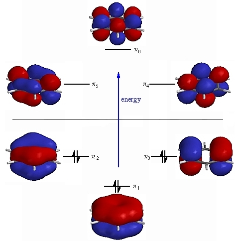