Rep:Mod:afm2015
Introduction to Molecular Dynamics Simulations
Molecular Dynamics is a technique used to study the behaviour and nature of atomic interactions, with respect to time. As we cannot computationally model entire large systems, approximations are made so we can examine the dynamics of smaller systems, and then scale up, within reason, to simulate the overall dynamics of the whole system. These approximations allow an accurate representation of the larger system providing that the number of atoms remains constant. By studying the atomic motion of the system and combining this with statistical mechanics on the microscale, we can compute properties on the macroscale. By considering the interactions between atoms, which previously in simpler approximations, would have been neglected, we can compute much more accurate data.
A good approximation is by treating particles in a system classically, with N atoms, all interacting with one another. By Newton's Second Law, we know that the force that each atoms exerts on another induces an acceleration, governed by the equation:
Where Fi = force acting on atom i
mi = mass of atom i
ai = acceleration of atom i
vi = velocity of atom i
xi = position of atom i
Computationally, it would be difficult to generate data for a system with a large number of atoms, due to the sheer quantity of different interactions occurring. This is why we use numerical solutions, such as the Verlet algorithm1 presented below, where the continuous function is broken up into small chunks, or timesteps. The Verlet algorithm is a very strong tool for molecular dynamics as it ensures the preservation of energy to a large degree. The Verlet algorithm also shows an error no greater than the fourth differential term. It does however require the initial position to be known, as well as the previous positions at the 'previous' timestep. It also does not allow the calculation of velocities, a required quantity for the calculation of properties of the system such as its energy. Hence, a variation known as the Velocity-Verlet algorithm2 is often used as it provides us with these essential details. This method does require the knowledge of the the initial positions as before, but also the initial velocity. As is known from statistical thermodynamics, the velocities of particles in a system is governed by the Maxwell-Boltzmann distribution and hence is relatively straight forward to determine at a given temperature.3
Using the Velocity-Verlet Algorithm
The Verlet algorithm is a method of discretising the molecular dynamics problem. By breaking up the continuous functions into discrete timesteps, we can numerically solve the equations to generate values for the physical properties of the system.
In addition to the equations above, the equation used in order to calculate the energy of the velocity-verlet solution was:
Where m = mass, v = velocity, k = spring constant and x = position.
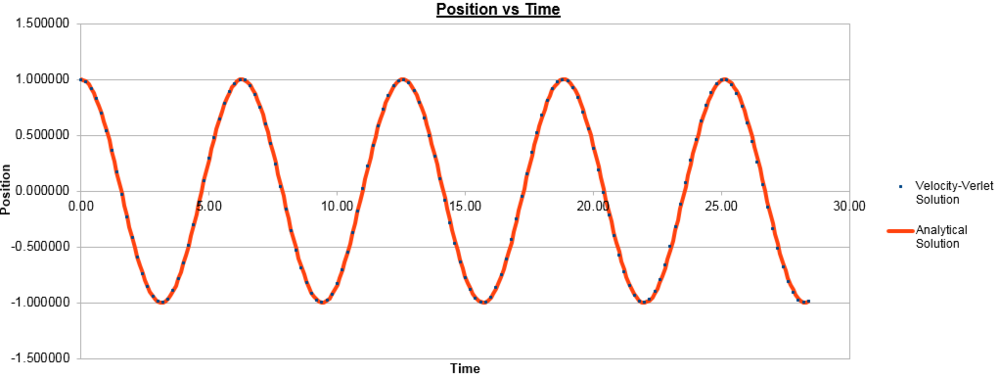
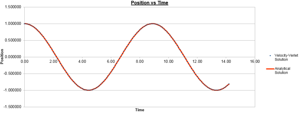
The initial conditions for the data below were:
k = 1, Timestep = 0.1000, Mass = 1.00, X(0) = 1.00, V(0) = 0.00, Phi = 0.00, A = 1.00, Omega = 1.00
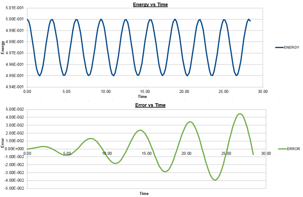
The timestep was subsequently changed to 0.2000 and the data below was generated:
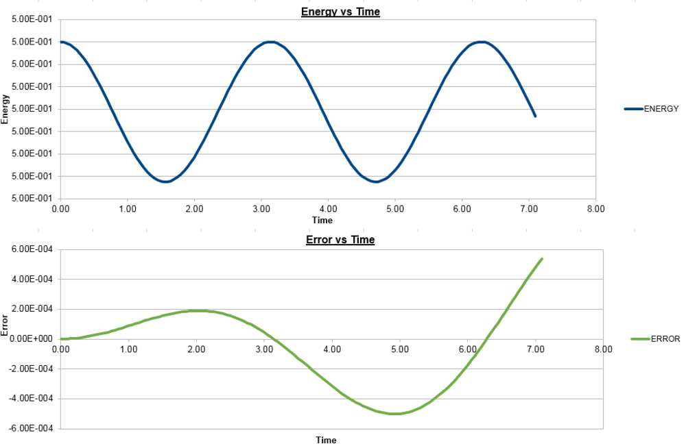
The timestep was then changed to 0.0500 to produce the following data:
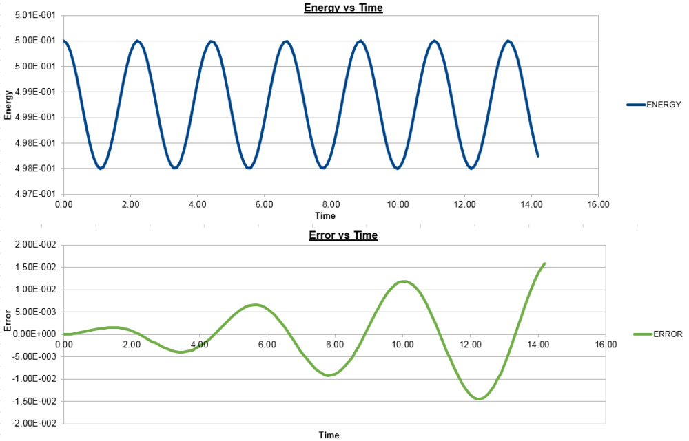
To ensure that the total energy does not change by more than 1% during the simulation, we need to make sure that the energy does not vary by more than 0.005, from the initial 0.5, so cannot go below 0.495. As can be seen in the graphs above, for the timestep of 0.2000, we see a 1% variation in energy. To demonstrate that an increased timestep increases the variation in energy, the graph for a timestep of 0.3000 is shown below.
It is important to monitor the total energy of the system when working numerically to ensure that the conservation of energy is being obeyed, and an accurate result is presented. If the energy fluctuates too greatly, this may be indicative of an error in the coding or the system not running to completion.
The error in the position changes with time as it does, with an increasing amplitude, due to the nature of the numerical solutions used to calculate the position and velocity. The faster the velocity and hence the change in position, the less accurate the Velocity-Verlet algorithm used is, as it is based on a Taylor expansion, which loses accuracy on larger time intervals. As the depiction of the error graph is based on the variations of the Velocity-Verlet solution, the increase in amplitude of the error curve is expected. With each subsequent change in position, there is an error involved, which cumulatively increases over the simulation, thus increasing the amplitude as the simulation progresses.
With all this in mind, the mass was changed in order to see what effect it had on each of the graphs.
For a mass of 2.00:
For a mass of 0.50:
As can be seen, by increasing the mass, the frequency of both position and energy curves decreases and vice-versa. This is to be expected as the frequency of oscillation of the harmonic oscillator is inversely proportional to the square root of the reduced mass. In this case, the reduced mass increases with the mass and hence the observed decrease in frequency, with the opposite true for decreasing the mass. It could also be shown that changing the spring constant has the opposite effect on the graphs, as the frequency is directly proportional to the square root of the constant and hence increasing the constant increases the frequency.
Using these boundary conditions along this vector for a single timestep, the atom ends up at (0.2, 0.1, 0.7).
Using the data above, the Lennard-Jones cutoff = 3.2 x 0.34 = 1.09 nm.
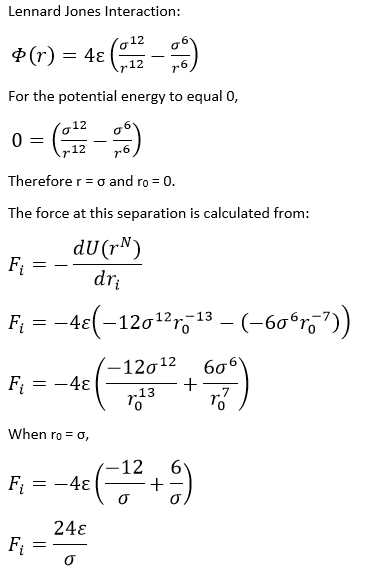
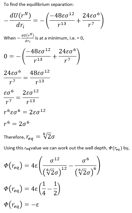
From previous calculations, the well depth = -ε, therefore:
Well depth = (120 x 1.38 x 10-23 x 6.022 x 1023) / 1000 = -0.997 kJ/mol
From Reduced Temperature = 1.5, and cancelling kB,
Temperature = 120 x 1.5 = 180 K
Equilibrium
Giving the atoms random starting coordinates causes problems as there is the potential for overlapping atoms, which besides having the obvious issue of impossibility, this will cause the potential between the atoms to be extremely high, and hence a large repulsion energy will be observed right at the start of the simulation. This will propel atoms far away from one another and therefore will not give an accurate representation of their equilibrium and will also cause the simulation to take much longer.
Volume = r3
= (1.07722)3 = 1.25
Number density = Number/Volume
= 1/1.25
= 0.8
For a face centered cubic lattice, N = 4.
Hence, 1.2 = 4/V
V = 3.33333
r = 3.333331/3
r = 1.494
If we had defined the lattice, this command would produce 400 atoms. This is calculated from the number of atoms per unit cell = 0.125 x 8 + 0.5 x 6 = 4. As we have 1000 unit cells, 4 x 1000 = 4000 atoms.
Mass 1 1.0
In the manual, this is denoted as Mass I Value where I is the atom type and value is the mass of the specified atom, I. This specifies that the mass of the atom type 1, is 1.0. If I is instead replaces by an asterisk, *, then all atom types from 1 to N, the total number of atom types, have the same mass, that which is listed in the 'value' section. An asterisk before a number, n, indicates atoms of type 1 to n have the 'value'. An asterisk after n indicates from n to N and a asterisk between two number indicates the 'value' between the two.
pair_style lj/cut 3.0
This is used to calculate 'pairwise interactions', potentials between atoms within a certain cutoff distance, in this case, 3.0. The lj part specifies Lennard-Jones, where coulombic interactions are ignored.
pair_coeff * * 1.0 1.0
The general structure of this is pair_coeff I J args, where I and J are the atom types and args is the coefficient for either of the atoms. It is used to specify the pairwise force field constants for the pairs of atom types.
We use the velocity-verlet algorithm, which is appropriate as we are specifying positions and velocities, as described before.
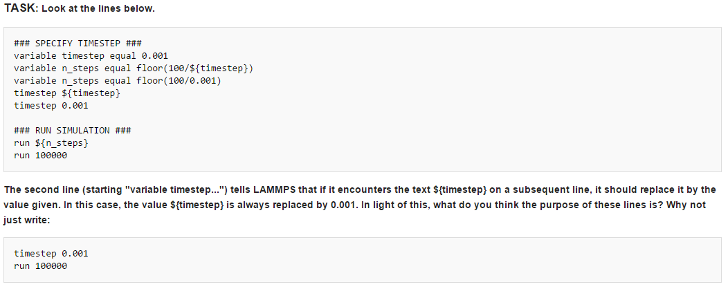
If the code were written in the simplified way as shown, each time we change the timestep, we would need to manually change the number of steps that are run in order to keep the overall simulation time constant, for each of the different timesteps. Otherwise, by doubling the length of the timestep, for instance, we would also be doubling the total simulation time. By using the floor function above, it enables us to simply change the timestep duration and the program will automatically reduce or increase the number of timesteps to be run in order to simulate the desired amount of time, keeping our x-axis of time constant throughout the simulations.
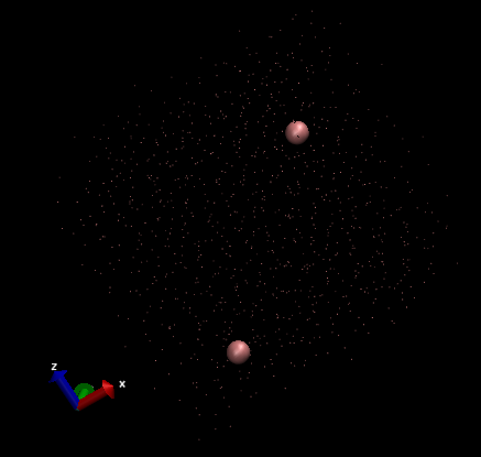
Shown below is a view of the total particles in the system:
And below here is a representation of just two individual particles.
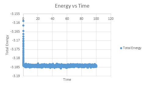
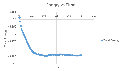
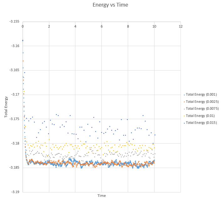
As can be seen, this system does reach equilibrium, which took approximately t = 0.4, visualised by altering the scale of the graphs, as seen below.
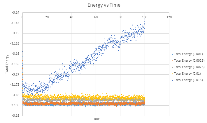
Finally, a single plot of Total Energy vs Time for each different timestep is shown below.
Of the five timesteps used, it is clear from the overlapping total energy vs time graphs that the largest timestep of 0.015 gives the bad result. From this graph it would appear that the other four tiemsteps give a similarly good result to one another but once the axes are expanded, we see this is not entirely the case.
As can be seen from this expansion of the graph, the two lowest timesteps of 0.001 and 0.0025 oscillate about a similar value, just above -3.185. With each increasing timestep, the total energy value increased, with a larger variation about its average also. In order to achieve the most accurate results, the oscillation amplitude about the average energy value needs to remain fairly small, so when the timestep is increased to 0.0075, already a decrease in accuracy is observed and hence the the largest to give acceptable results in this case is the 0.0025 timestep. This provides the necessary trade off between accuracy and the time we can simulate of the system.
Running simulations under specific conditions
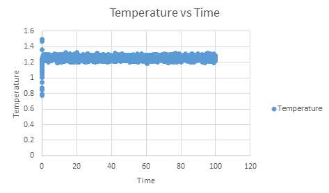
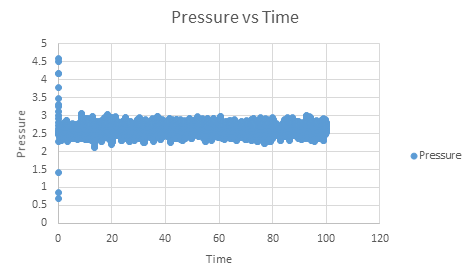
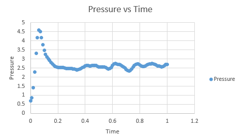
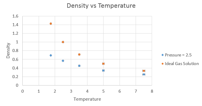
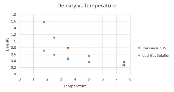
The temperatures chosen were 1.75, 2.5, 3.5, 5 and 7.5. These are all above the critical temperature but not significantly so, but will still give a nice range of values. The pressures used were chosen by looking at the pressure vs time graph above. It can be seen that the pressure is at an equilibrium of about 2.5, and hence values similar to this of 2.5 and 2.75 were chosen. Ten simulations were run, each temperature at the two different pressures. The timestep was chosen to be 0.001, which as seen before, gave the most accurate results.
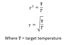
By simply diving the second equation by the the first equation, we are left with:
The three numbers above are important because they let you know how the average properties are to be calculated. The line they are present in tells the program to take a sample every 100 steps, to take 1000 samples in total, and to do this until 100000 timesteps have passed, before calculating an average of each of the properties being determined. The 100000 is therefore governed by the previous two values, and requires them in order to be complimentary of itself. The following line states "run 100000" which stipulates that the process will be run for 100000 timesteps.
The equation used to plot the results from the ideal gas law was pV = NkBT, rearranged to N/V = p/kBT. The results were as follows.
The simulated density is lower than that of the ideal gas law. In the ideal gas law, we assume there is no potential energy in the system and hence the atoms come closer together, with a smaller equilibrium distance between them, which leads to the higher density. This close approach is not possible when we consider the potential interactions, which while small between individual atoms, do build up in larger systems. This is amplified by the strong distance dependency on the repulsive term in the Lennard-Jones potential, where at very small distances, the repulsion is extremely strong.
As the pressure was increased, the discrepancy between the ideal gas law and the simulated result increased. This is to be expected, as the simulation takes into account the potential interactions between atoms, which increase on the increase in pressure. The ideal gas law is a good approximation for when the atoms are far apart and hence not interacting to any real degree, but breaks down when atoms are close enough to have significant interactions between one another.
Calculating heat capacities using statistical physics
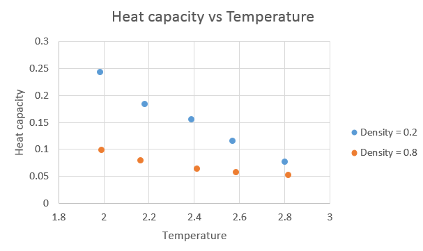
The graph below shows a plot of the heat capacity against temperature.
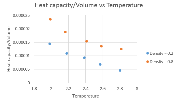
The next graph shows heat capacity divided by volume against temperature.
The trend is as expected, with the heat capacity increasing with increasing density and decreasing as the temperature increased. As the amount of atoms in the "box" is constant, on increasing the density, we decrease the volume. For a density of 0.2, the volume was 16875 and at a density of 0.8, the volume was 4219. With a greater number of atoms in the same space, the larger the expected heat capacity in that volume is. As each atom contributes a set amount to the heat capacity, hence with more atoms in the smaller volume, the higher the heat capacity will be when associated with that volume. As the temperature is increased, higher thermal energy levels become occupied, and therefore lose some of their "capacity" to absorb "heat" energy, and hence the observed decrease in heat capacity. Intuitively, this would lead to the assumption that the heat capacity will tend to zero as the temperature tends to infinity.4
Structural properties and the radial distribution function
The temperatures and densities were chosen from the provided journal article5 and are as follows:
Vapour: Density = 0.05, Temperature = 1.25
Liquid: Density = 0.8, Temperature = 1.25
Solid: Density = 1.1, Temperature = 1.25
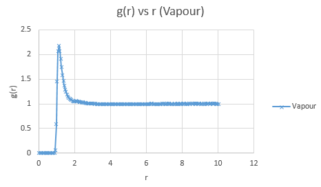
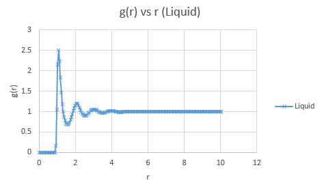
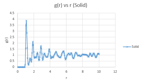
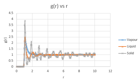
Below are presented the g(r) radial distribution function graphs for vapour, liquid and solid in turn.
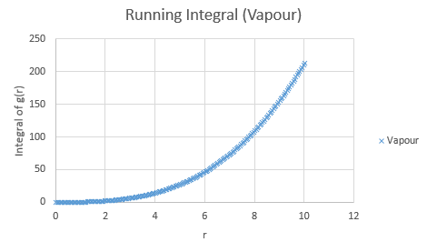
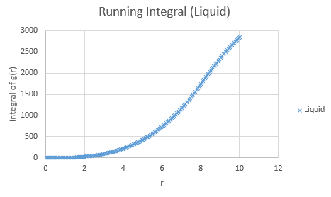
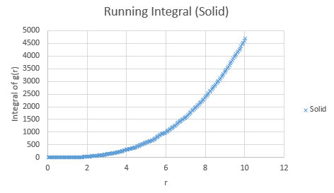
Below are the running integrals of each of the functions.
Qualitatively, from these graphs, we can determine how ordered a system is and where its defects lie. Solids, liquids and gases are all very different systems and hence show different radial distribution functions. The radial distribution function tells us how the atoms are distributed, their dispersion density, as a function of radius, which can be thought of as a comparison between the system close to an individual atom, and the overall system itself. The large number of peaks in the solid spectrum are due to its highly ordered close range structure where very little deviation is allowed. The liquid shows much fewer peaks, but still some, due to its slight ordering but greater variable movement than the solid phase, and the vapour phase shows even less due to the highly disordered random motion it undergoes.
The peaks we see in the spectra indicate the preferred equilibrium distance between atoms. For the solid state, the deviations we see are due to imperfections in the face centered cubic (FCC) crystal packing it exhibits, and hence we do not see the strictly ordered peaks we would expect from a perfect cubic structure. Due to the random Brownian motion occurring in the fluids, the preferential distance between atoms does not vary as significantly due to all the various collisions taking place. As time progresses we see a decline in g(r) to an actual equilibrium value, which occurs more rapidly in the fluids than the solid. This is as expected as any defects in the solid lattice will take longer to stabilise in position, as their motion is purely vibrational, with no large scale significant collisions occurring. With regards to the solid state, it is to be expected that any slight deviations cause a large spike in the radial distribution function, as the majority of the crystal is highly ordered, so the short range discrepancy will be significant, even if the deviation is only small. Therefore the pattern of decreasing variability of the function is also expected, as the overall order is decreasing with distance and hence the general structure of the crystals at a greater distance will not vary as significantly from small deviations. Our function is also only accurate up to a certain degree and therefore at longer ranges than the error present is feasible for where finding a defect is statistically likely, we see a broadening and flattening of the peaks associated with it.
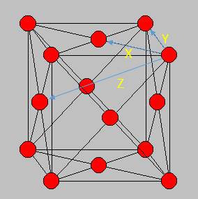
Entropically, having defects in the crystal is actually a favoured process, with an increased number of microstates available and hence perfect crystals are difficult to produce. The peak structure seen would be indicative of its FCC structure, and if the crystal structure was different e.g. body centered cubic, then the distribution function would look slightly different. The first three peaks can be allocated to specific lattice points in the FCC structure, corresponding to the smallest distances between atoms in the lattice. The smallest distance, denoted x, corresponds to the first peak, y, the second peak and z the third peak. These are shown in the figure below.
The lattice spacing can be approximately determined from the solid graph. As we are in an FCC lattice, we know that the distance Y, above, to our chosen atom is a single lattice parameter away and by looking at the second maxima, we see this is at r = 1.525. The coordination numbers for each of the first three peaks can be determined by comparing where the peaks begin to decrease, to the running integral graph. The first peak diminishes at r = 1.325, which corresponds to the running integral value of 12.11 on our graph and hence a coordination number of 12. The second peak does so at 1.675, corresponding to approximately 18 on the running integral curve, so by subtracting the first peak value, we obtain 6 as its coordination number. Finally the third peak does so at r = 2.075 and a running integral of 44. Similar to previously by minusing the first two peaks, we obtain a coordination number of 26. These numbers are based purely off the obtained graphs and hence are only approximations, as the values have not been fully extrapolated to produce the most accurate values.
Dynamical properties and the diffusion coefficient
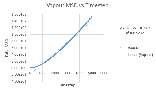
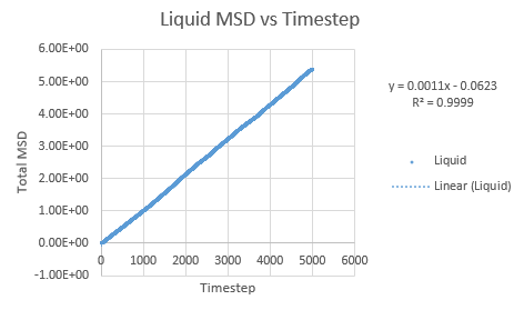
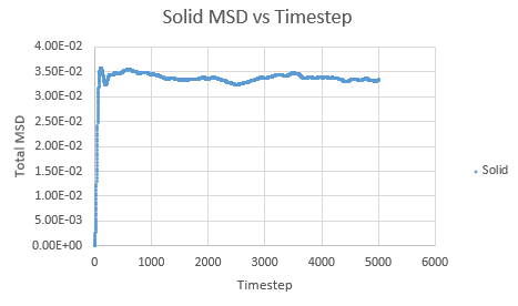
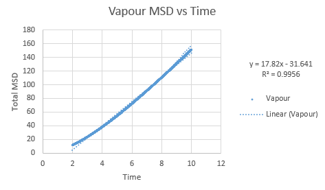
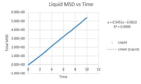
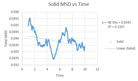
Simulations were performed in order to ascertain the mean squared displacement (MSD) of each state, solid, liquid and vapour. These in turn can then be used to calculate the diffusion coefficients. Graphs of these MSD's are shown below.
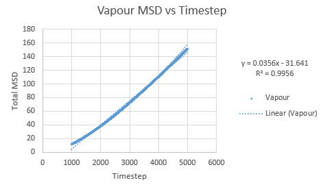
As this curve does not show linearity initially, a regression line was plotted from different timesteps until a greater linearity was achieved.
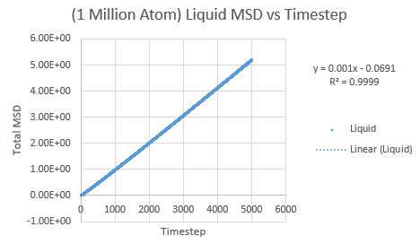
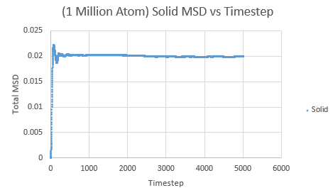
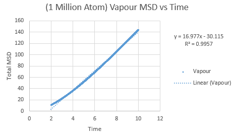
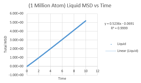
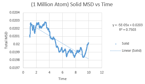
The trend in these curves shown above is as expected, with both vapour and liquid showing an apparent linear relationship. We expect the atoms to be undergoing random Brownian motion, collides randomly with atoms around it. It is evident however that the vapour phase does not start off linearly, as at the start of the simulation in the low density vapour phase, the atoms are far apart and hence very few collisions occur initially, with atoms in fact moving with a constant velocity. This introduces a distance dependence into the simulation, which is only overcome after several timesteps have passed. The "squared" nature of MSD is what gives the start of this curve its apparent parabolic trajectory. The liquid showed the expected linearity right from the start of the simulation, as the atoms are a lot closer together to start with and hence collisions begin occurring much more readily. The solid graph on the other hand shows a completely different trend, sharply increasing initially and then leveling off. This initial sharp increase is indicative of the nature of solid crystals, where the atoms are very closely packed together and hence do not have a lot of space to move around in. At the start of the simulation, the atoms spread out in their own individual space, appearing to explore the surroundings, but once this has occured, there is nowhere else for the atoms to go, their displacement can no longer change significantly and hence the curve flattens off. To determine the slope of this curve, the initial sharp increase was ignored and the linear part analysed.
In order to calculate D, the diffusion coefficient, the timestep graphs were converted into time. The slope of each line was then used to determine D for each state.
Slope of vapour curve = 17.82
D = 2.97
Slope of liquid curve = 0.5451
D = 0.09085
Slope of solid curve = -9 x 10⁻⁵
D = -1.5 x10⁻⁵
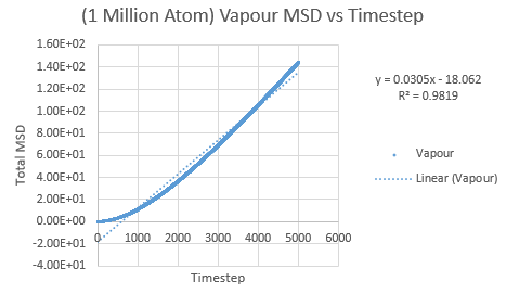
The same was then conducted on the provided 1 million atom systems, giving the graphs as follows.
Slope of vapour curve = 16.977
D = 2.8295
Slope of liquid curve = 0.5236
D = 0.08727
Slope of solid curve = -5 x 10⁻⁵
D = -8.3 x10⁻⁵
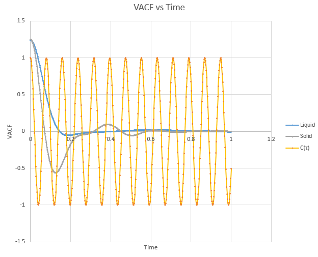
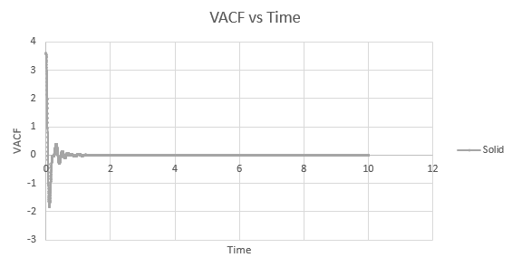
Shown below is a plot of the velocity autocorrelation functions for the liquid and solid simulations, and the heat capacity as derived above, in 1-dimension.
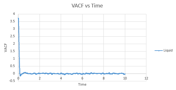
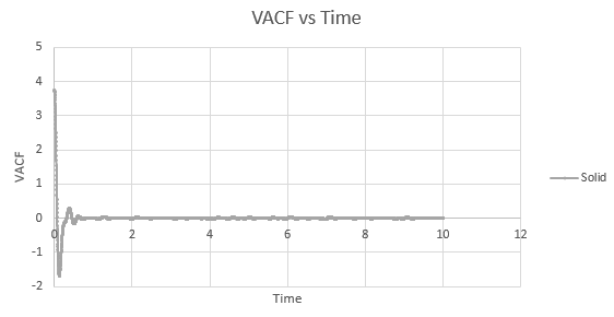
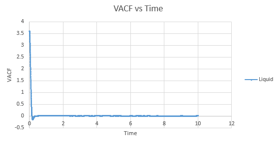
The minima in the solid and liquid VACF's represent the point at which the vectors of velocity are parallel in opposite directions, so that the difference between velocities at the two respective times is minimised. This occurs when the atoms collide with each other and so directly after have velocity vectors opposite to one another. In a liquid this is more emphasised than in a solid, as the atoms are allowed to diffuse from each other also, and hence are allowed greater velocity vectors than in the solid.
The observed differences between the solid and liquid VACF's are explained due to the difference in atomic motion allowed in the systems. The liquid system has a much less strict structure and atoms are constantly diffusing around the system, whereas in a solid the movement is purely vibrational. Each of the atoms is aiming to be in its equilibrium position which minimises the interaction energies with the atoms around it. In a solid, this position is more readily achieved, due to the strictly ordered nature of its structure. The solid graph shows what appears to be a continuous oscillation about zero, which can be rationalised due to the persistent 'jostling for position' the atoms in the lattice will exhibit, continually changing velocity vector. In the liquid system, diffusion overpowers these oscillations fairly swiftly, damping it significantly and leading to a curve which tends to zero quite quickly with only a single apparent minima. As time progresses, the solid system will also tend to zero as the magnitude of oscillations decreases.
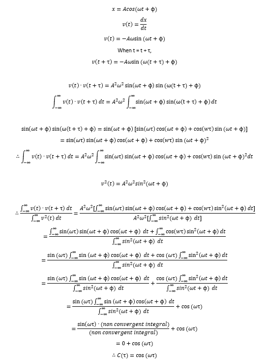
The harmonic oscillator VACF is very different to the Lennard-Jones, mainly due to the Lennard-Jones' non-symmetric nature, whereby the 'left side' nearest to t = 0 is a lot more variable than the function at later times. The harmonic oscillator is not influenced by the changes in velocity and hence stays fully symmetrical, whereas in the VACF, the function C(τ) will decrease with changing velocity, so the VACF systems show a strong damping effect unlike a harmonic oscillator.7
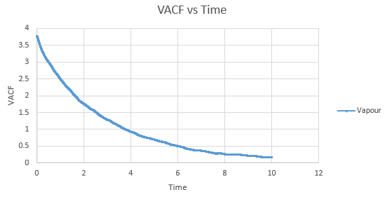
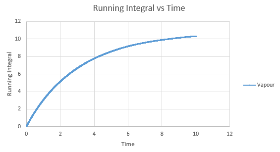
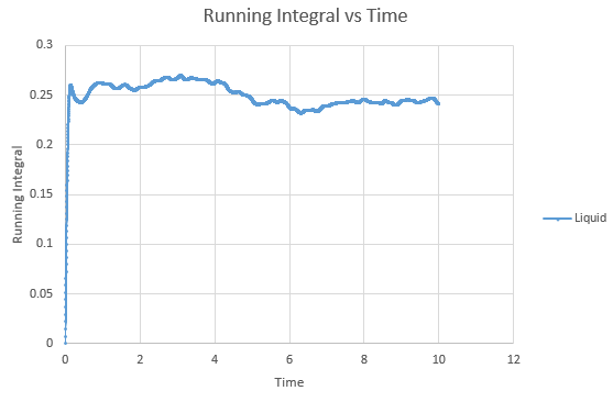
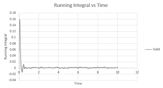
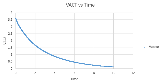
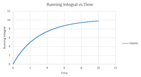
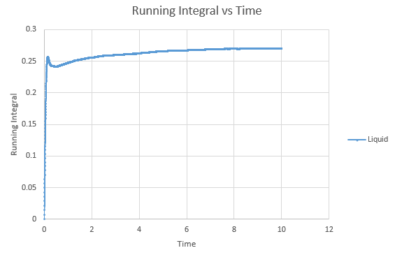
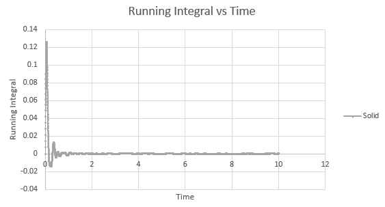
Shown below are the individual VACF plots for each vapour, liquid and solid in turn, and their corresponding running integral curves, determined via the trapezium rule.
Vapour:
Diffusion coefficient, D = 3.443
Liquid:
D = 0.08036
Solid:
D = 5.59 x 10⁻⁴
Doing the same process for the million atom simulations:
Vapour:
D = 3.268466
Liquid:
D = 0.090091
Solid:
D = 4.55 x 10⁻⁵
On the whole, the running integrals are as expected. The diffusion coefficients obtained from the final value on the graphs show a decent correlation the the diffusion coefficients calculated in a previous section. The largest source is error is likely to come from the limitations of the trapezium rule, which is inherently less accurate the less trapezoids are used. The larger the deviation in the line from linearity within each of the trapezium regions, the less accurate it becomes, and as our lines show significant curvature, this error is likely to build up. In this case due to the sheer number of trapeziums used, the method is a good approximation to calculate the diffusion coefficients from, as shown by their relative closeness to the values from our MSD calculations.
Conclusion
In this experiment, we have successfully shown how different methods can be used to simulate various properties in fluid and solid systems. By simulating on the microscale, we have been able to compute macroscopic properties of the systems, and show correlations between different, yet equally valid, methods.
References
1. L. Verlet, Phys. Rev., 1967, 159, 98-103.
2. W. C. Swope, H. C. Andersen, P. H. Berens and K. R. Wilson, J. Chem. Phys., 1982, 76, 637-649.
3. J. C. Maxwell, Philosophical Magazine, 4th series, 1860, 19, 19-32.
4. http://people.virginia.edu/~lz2n/mse209/Chapter19c.pdf (Accessed: 20/03/2015).
5. J. Hansen and L. Verlet, Phys. Rev., 1969, 184, 151-161.
6. http://ecee.colorado.edu/~bart/book/fcc.gif (Accessed: 23/03/2015).
7. http://people.virginia.edu/~lz2n/mse627/notes/Correlations.pdf (Accessed:24/03/2015).
