
Rep:Mod:adt103
Modelling Transition States in Organic Chemistry
Module 1: Modelling the Transition State in the Cope Rearrangement
Introduction

The Cope rearrangement is an example of a [3,3] Sigmatropic rearrangement that occurs in 1,5-substituted dienes. The Cope rearrangement widely agreed to be a pericyclic reaction and therefore occurs in a concerted fashion. The exact nature of the mechanism for the reaction was however for some time the subject of much debate and because pericyclic reactions proceed without any intermediates in the reaction co-ordinate; we are able to model them with a high degree of accuracy.
The transition states under investigation are shown in Scheme 1 and are believed to adopt either a chair or boat like structure. Similar to that of the conformations of cyclohexane, the boat transition state is a higher energy pathway than that of the chair transition state. In order to quantify the different energies involved in these transition states we need to model the reaction using Gaussian. In order to work out the energy of the transition state however we need to establish the most thermodynamically stable conformation of 1,5-hexadiene, i.e. the one with the lowest energy.
Optimisation of 1,5-hexadiene
Advances in computational chemistry has allowed us to model molecules and optimise their geometries with speeds and accuracy unthinkable only a few decades ago. A simple hydrocarbon such as 1,5-hexadiene, C6H10, can adopt many different conformations differing only in the orientation of a handful of atoms. It is the difference in energy between these isomers that can be calculated using Gaussian. We can start the optimisation process by using a crude method to separate out the highest energy conformers, eventually using higher level calculations to ascertain the lowest energy isomer. We shall start with the Hartree-Fock method using a 3-21G basis set. From the optimised structures obtained we can identify any symmetry elements associated with individual isomers, the results are shown in Scheme 2.
| Conformer | Point Group | Energy (Ha) | Energy (kcal/mol) | Energy difference (kcal/mol) |
| Gauche 1 | C2 | -231.68771616 | -145386.2429 | 3.1031 |
| Gauche 2 | C2 | -231.69166694 | -145388.7221 | 0.6239 |
| Gauche 3 | C1 | -231.69266122 | -145389.3460 | 0.0000 |
| Gauche 4 | C2 | -231.69153035 | -145388.6364 | 0.7096 |
| Gauche 5 | C1 | -231.68961570 | -145387.4349 | 1.9111 |
| Gauche 6 | C1 | -231.68916016 | -145387.1490 | 2.1970 |
| Anti 1 | C2 | -231.69260213 | -145389.3089 | 0.0371 |
| Anti 2 | Ci | -231.69253511 | -145389.2669 | 0.0791 |
| Anti 3 | C2h | -231.68907066 | -145387.0929 | 2.2531 |
| Anti 4 | C1 | -231.69097051 | -145388.2851 | 1.0609 |
From Scheme 2 we can see that there are three conformers that are similarly low in energy - Gauche 3, Anti 1 and Anti 2.

One would expect the Anti conformations to be the lowest in energy because the large R-groups are anti-periplanar. Although both the Gauche and Anti conformations are eclipsed the Gauche conformations suffers repulsion due to the steric encumbrance of the two R-groups next to each other and hence one would presume this would be higher in energy (Scheme 3). From the results in Scheme 2 we can see that in fact the Gauche 3 conformer is the most stable due to a favourable interaction between the two alkene π-orbitals in the (HOMO) (Scheme 4) and the π-orbital and vinyl proton [1]. One key factor that we have not taken into account however is the accuracy with which the values were predicted. The HF/3-21G optimisation, whilst giving us a good idea of the lowest and highest energy conformations, is not accurate enough within the margin or error that we are dealing with in these lowest energy conformers. In order to check these results we need to perform another optimisation but instead using a more advanced method - DFT/B3LYP and basis set - 6-31G(d). The results of the optimisation are shown in Scheme 5.
| Conformer | Point Group | Energy (Ha) | Energy (kcal/mol) | Energy difference (kcal/mol) |
| Gauche 3 | C1 | -234.61132932 | -147220.8380 | 0.2955 |
| Anti 1 | C2 | -234.61180027 | -147221.1335 | 0.0000 |
| Anti 2 | Ci | -234.61171457 | -147221.0797 | 0.0538 |
While the overall structural geometry has not changed significantly because the point group is identical we can see from Scheme 5 that the relative energies of the conformers has changed. The more advanced calculation has rendered the Anti 1 conformation almost 0.3 kcal/mol lower in energy than the Gauche 3 conformer. This change highlights the advantage of using a more complex method and basis set in determining the energies resulting from the small structural changes in conformational isomers. However even the DFT/B3LYP 6-31G(d) method and basis set does not locate the true global minima. It has been shown that no definitive lowest energy conformation can be found, with different methods giving contradictory results. The Hartree-Fock method is a weak method of structural optimisation because it neglects electron correlation, treating the conformations similar to those of n-butane. What is demonstrated is that there is very little difference in energy between the Anti- and Gauche- conformations, an order of magnitude less than the Anti- and Gauche- conformations in n-butane [2]. The only way of determining a true global minima is to yet increase the complexity of the method and use a larger basis set for the calculation. Unfortunately we are not going to investigate the energy differences between the conformations further in this project although it is an interesting and unsolved mystery.
Frequency analysis at the DFT/B3LYP level of the Anti- 2 conformer of 1,5-hexadiene
As with the HF method, the DFT/B3LYP method does also not take into account certain other factors. An additional frequency calculation at the same level as the optimisation must be carried out. The frequency calculation takes into account thermal energy and enthalpy and the results are shown in Scheme 6.
| Temperature (K) | Eelec + ZPE (Ha) | E + Evib + Erot + Etrans (Ha) | RT (H = E + RT) (Ha) | Entropic contribution to the free energy (G = H - TS) (Ha) |
| 0 | -234.469214 | -234.469214 | -234.469214 | -234.469214 |
| 1 | -234.469214 | -234.469204 | -234.469201 | -234.469234 |
| 298.15 | -234.469214 | -234.461865 | -234.460921 | -234.500798 |
| 521.15 | -234.469214 | -234.449762 | -234.448111 | -234.534171 |
The values shown in Scheme 6 are the results of the frequency analysis using the DFT/B3LYP method with a 6-31G(d) basis set. The results show a variety of thermodynamic and electronic contributions to the energy. The first contribution calculated is the sum of the electronic and zero point vibrational energy (ZPE) at 0K - Eelec + ZPE. The second quantity calculated is the sum of the electronic and thermal energies, the thermal energies include vibrational, rotational and translational energies - E + Evib + Erot + Etrans. The third quantity calculated is the sum of the electronic and thermal enthalpies. This particular result takes into account a correction for the measurement at room temperature - RT (H = E + RT). The fourth quantity is the sum of the thermal and electronic free energies. This result includes an entropic contribution to the free energy - (G = H - TS). The results at 0K are all equal because all of the thermal energy and enthalpy terms are equal to zero, therefore only the ground state electronic term results. This is verified by running the calculation just above zero at 1K, here we see that the population of the thermally accessibly states is barely large enough to register above 4 d.p. The result the for the first term, Eelec + ZPE is the same regardless of temperature and equal to the result at 0K as this represents the ground state energy when no thermal population of higher levels occur and is close to that reported in literature of -234.46925 [3]. The results also give rise to the IR stretches of the alkenes - 1731.25cm-1 for the symmetric and 1734.50 for the asymmetric stretches.
Optimising the chair and boat transition states
Modelling the chair transition state using the Berny method
Now that we have established the optimised structures and energies of 1,5-hexadiene we can model the transition states of the Cope rearrangement. In order to do this we have to first construct an allyl fragment and optimise it to the HF/3-21G level. We construct an allyl fragment because this represents one half of the transition state whereby the double bond character is split over the entire structure. Once the structure is optimised and is of C2v symmetry, two allyl fragments can me modelled approaching each other in an approximate chair conformation. It is important that the initial modelling is close enough to the actual transition state otherwise the calculation will not work. The calculation produces a force constant matrix known as the Hessian, this however depends on the curvature of the so-called reaction co-ordinate. As the reaction proceeds through the transition state this curvature should appear negative however if the initial structure is far removed from the actual transition state then the curvature may vary too widely and hence not work. In order to initially model this we are going to set the two terminal carbons of the allyl fragments 2.2Å apart. The optimisation and frequency calculation was run using again the Hartree Fock method with a 3-21G basis set optimising to a Berny transition state calculating the force constants once. The results are best manifested by the vibration of the transition state seen (here). The frequency of this imaginary vibration occurs at -817.85cm-1 and the equilibrium distance between the two terminal carbons is 2.27Å. The calculation was repeated again but this time using a more complex DFT method and large 6-31G(d) basis set. The frequency of this imaginary vibration occurs at -565.54cm-1 and the equilibrium distance between the two terminal carbons is 1.98Å, the vibration of the transition state seen (here). The results are shown in Scheme 7.
N.B. When calculating the TS(Berny) from a guessed structure it is necessary to add Opt=NoEigen to the Gaussian calculation input so that the calculation does not terminate if more than one imaginary vibration is found during the optimisation.
| Optimised chair TS(Berny) HF/3-21G | Optimised chair TS(Berny) DFT/6-31G(d) | |||||||
| Structure |
|
| ||||||
| Frequency of vibration (cm-1) | -818.85 | -565.54 | ||||||
| Equilibrium C-C distance (Å) | 2.27 | 1.98 |
Modelling the chair transition state using the frozen co-ordinate method
Another method of modelling the chair TS is by using the frozen co-ordinate method, this procedure freezes the position of the two bonding atoms until the optimisation has been completed on the rest of the molecule. After the other parts of the molecule have come to rest at their minima the remaining atoms are unfrozen and the optimisation then proceeds to the transition state (Berny) again using the HF method and 3-21G basis set. This method does have some distinct advantages over calculating the entire Hessian matrix in one fell swoop if the derivatives of the calculation along the reaction co-ordinate are close enough to the real force constant matrix.
To calculate the chair TS using this method we start again with the two allyl fragments but first freezing the co-ordinates of the bonding carbons in the allyl fragments. An optimisation is run at the HF/3-21G level and then the co-ordinates of the bonding carbons unfrozen and instead set to differentiate along the reaction co-ordinate. This is then run again at the HF/3-21G level. The results of the calculation are very similar to those of the chair TS using the previous Berny method. The frequency of vibration at the TS occurs at -817.90cm-1 and the equilibrium distance between the terminal carbon atoms is 2.02Å. The vibration of the chair TS can be seen (here). The calculation was repeated again but this time using a more complex DFT method and large 6-31G(d) basis set. The frequency of this imaginary vibration occurs at -565.46cm-1 and the equilibrium distance between the two terminal carbons is 1.97Å, the vibration of the transition state seen (here). The results are shown in Scheme 8
| Optimised chair TS(Berny) HF/3-21G | Optimised chair TS(Berny) DFT/6-31G(d) | |||||||
| Structure |
|
| ||||||
| Frequency of vibration (cm-1) | -817.90 | -565.46 | ||||||
| Equilibrium C-C distance (Å) | 2.02 | 1.97 |
One can see that from Schemes 7 and 8 the vibrational frequencies of the HF methods and DFT methods are very similar for both processes and overall the equilibrium bonding distances are very similar. The results of the equilibrium bonding distances for the frozen co-ordinate method are much closer than those using the Berny force constant matrix method, this is indicative of the potential problems that can be encountered when using this method if the initial approximation is too far away from the actual transition state.
Optimising the boat transition state using QST2 method
Now that we have considered the chair transition state we can model the boat transition state. In order to do this we shall use a new method - QST2. The QST2 method requires us to map the atoms of our reactant 1,5-hexadiene onto our product 1,5-hexadiene and then the calculation provides an associated transition state. We first start by using our DFT/B3LYP/6-31G(d) optimised anti-2 diene conformation as both the product and reactant, however we must label the atoms accordingly from the reactant molecule to where they end up in the product molecule (Scheme 9).

The optimisation and frequency calculation is performed at the HF/3-21G level optimising to a QST2 TS however taking the optimised diene and simply performing the calculation does not provide the anticipated result (initially proposed TS see here). The calculation does not proceed as expected because the calculation merely interpolates linearly along the reaction co-ordinate translating the reactant molecule into the product. In order to arrive at the boat TS we need to alter the structure of our reactant and product molecules to something resembling the TS more closely. We first alter the central dihedral angle (C2 to C5) to 0o and the bond angle (C2 to C4 and C3 to C5) to 100o (Scheme 10).

When the same calculation is performed on these modified reactants and products the result is something which closely resembles the desired boat TS (here). The frequency of vibration at the TS occurs at -840.79cm-1 and the equilibrium distance between the terminal carbon atoms is 2.14Å. The calculation was repeated again but this time using a more complex DFT method and large 6-31G(d) basis set. The frequency of this imaginary vibration occurs at -530.59cm-1 and the equilibrium distance between the two terminal carbons is 2.21Å, the vibration of the transition state seen (here). The results are shown in Scheme 11.
| Optimised boat TS(QST2) HF/3-21G | Optimised boat TS(QST2) DFT/6-31G(d) | |||||||
| Structure |
|
| ||||||
| Frequency of vibration (cm-1) | -840.79 | -530.59 | ||||||
| Equilibrium C-C distance (Å) | 2.14 | 2.21 |
The Intrinsic Reaction Co-ordinate
The Intrinsic Reaction Co-ordinate (or IRC for short) allows us to view how the structure of the molecules change from the high energy transition state along the potential energy surface to the product and reactant. The IRC is very powerful in so much as it allows us to see the path taken from product to reactant and how many transition states it passes through by taking many points and slightly modifying their geometry so it goes down in energy along the potential energy surface. For the Cope rearrangement we have studied, the product and reactant are exactly the same molecule and so we would expect there to be no change in the overall energy of the system. In addition to this, because the reaction is pericyclic we should expect a smooth transition state with no high energy intermediates, which would indicate an asynchronous non-pericyclic reaction. Scheme 12 shows how the various reaction profile diagrams vary with the expected energy profile diagram for the Cope rearrangement of 1,5-hexadiene.

We are going to look at the IRC for the HF/3-21G optimised chair transition state. It is important to note at this stage that the IRC calculation must be performed at the same HF/3-21G level as the TS optimisation because otherwise they will start from a different point on the potential energy surface. There are a few different ways of calculating the IRC but we are going to focus on two, calculating the force constants once, and calculating them at every stage. As we are inputting the transition state, i.e. the highest energy configuration, we should expect for the IRC to be a smooth slope down in energy towards the lowest energy Gauche-3 conformation of 1,5-hexadiene as calculated in section 2.2. Because the product and reactant are identical we could in theory calculate the IRC in any direction (forward or backward) from the transition state and end up with the same result. For fullness however we shall calculate the IRC over the entire reaction.
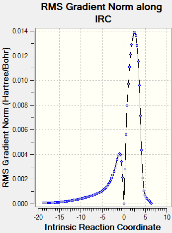
Calculating the force constants once at the start of the calculation is the least accurate method of plotting the IRC and the results are seen in Scheme 13.

The RMS gradient IRC can be seen (here). The calculation resulted in the formation of 47 reference points and there individual energies can be seen (here). From inspection of the individual results the reaction profile is not symmetrical and the energy of the product and reactant differ by 1.7 kcal/mol. By visual inspection there is very little difference in geometry between the product and reactant. A more accurate result is achieved through instead of calculating the force constants at every point instead of just once. The results of this are shown in Scheme 14.

The RMS gradient IRC for the force constants calculated at every stage can be seen (here). The calculation resulted in the formation of many more reference points, 87 in total and the individual energies can be seen (here). Calculating the force constants at every point leads both sides of the transition state to the same minima as expected. The geometry of the product and reactant can be seen (here). The point group of the product/reactant is C2 and they are both adopting the same Gauche-2 conformation. Scheme 15 shows an animation of how the structure changes as it passes along the potential energy surface.

It is expected that the potential energy surface would find the minimum at the Gauche-3 conformation which was calculated to be the lowest in energy at the HF/3-21G level but instead has found the Gauche-2 conformation. It is clear however that the conformation of the product/reactant is not the same energy as that calculated in section 2.2 but does possess the same symmetry elements and so we can conclude that conformation is somewhere between the conformations of the Gauche 2 and Gauche 3 diene. Scheme 16 shows a small results table comparing the data of the two methods.
| Force constants calculated- | Number of reference points | ΔE transition (kcal/mol) |
| once | 47 | 43.5 to reactant, 41.8 to product |
| at every point | 87 | 45.3 to both |
As we can see from Scheme 16, calculating the force constants only once leads us to reactants and products of different energy highlighting the unreliable nature of using this method. Calculating the force constant at every point allows a true minimum to be found, confirmed by the identical activation energies.
Results of Activation Energies
After conducting many calculations it is difficult to see how the different methods compare to the values found experimentally. A summary is shown below where the boat and chair transition states are compared in energy to the anti-2 conformation of 1,5-hexadiene.
Summary of energies (in hartree)
| HF/3-21G | B3LYP/6-31G(d) | |||||
|---|---|---|---|---|---|---|
| Electronic energy | Sum of electronic and zero-point energies | Sum of electronic and thermal energies | Electronic energy | Sum of electronic and zero-point energies | Sum of electronic and thermal energies | |
| at 0 K | at 298.15 K | at 0 K | at 298.15 K | |||
| Chair TS | -231.619322 | -231.466703 | -231.461344 | -234.556983 | -234.414930 | -234.409009 |
| Boat TS | -231.602801 | -231.450923 | -231.445293 | -234.543091 | -234.402342 | -234.396004 |
| Reactant (anti2) | -231.692535 | -231.539539 | -231.532568 | -234.611715 | -234.469214 | -234.461865 |
The activation energy can be calculated from the difference in energy between the TS and corresponding ground state molecule. This was done at 0K and 298.15K. The results of the activation energies are shown below:
Summary of activation energies (in kcal/mol)
| HF/3-21G | HF/3-21G | B3LYP/6-31G* | B3LYP/6-31G* | Expt. | |
| at 0 K | at 298.15 K | at 0 K | at 298.15 K | at 0 K | |
| ΔE (Chair) | 45.70 | 44.69 | 34.06 | 33.17 | 33.5 ± 0.5 |
| ΔE (Boat) | 55.61 | 54.77 | 41.96 | 41.33 | 44.7 ± 2.0 |
Experimental values[4]
From the results of the activation energy calculations two things are clear. The boat transition state has consistently a higher activation energy than the chair transition state and the DFT/B3LYP/6-31G(d) calculations are much closer to the experimental values. The fact that the boat is the higher energy transition state should not come as any surprise and can be inferred from the conformational energy analysis of cyclohexane. Interactions between the two flagpole hydrogens generates significant steric strain in the system meaning that the chair conformation is energetically favoured. The activation energy calculated at 298.15K at the DFT/B3LYP level for the chair conformation is well within the experimental error whereas the same energy calculated at the HF/3-21G level is over 10kcal/mol out. This reinforces that even a small improvement in the method and a larger basis set can drastically improve the calculation results.
Diels-Alder cycloaddition reactions
Introduction

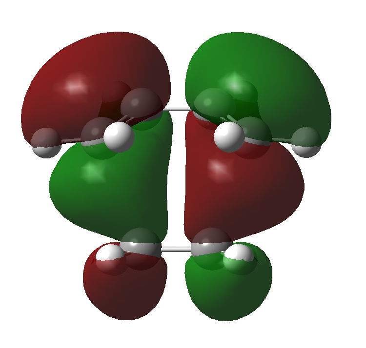
The Diels-Alder reaction was discovered over 80 years ago and remains one of the most powerful methods for synthesising 6-membered rings with high degrees of stereo- and regioselectivity. The Diels-Alder reaction is a π4s + π2s cycloaddition reaction involving two components a 1,5-diene and an alkene called the dienophile. The combination of these two parts can form heavily substituted 6-membered cyclohexene rings. There are several important factors that must be considered when looking at the Diels-Alder reaction, namely the conformation of the diene, the substitution of the dienophile and the resulting stereochemistry of the product. In order for the reaction to take place the diene must be in the s-cis conformation and ideally the dieneophile electron poor. The necessity for the electron deficiency in the dienophile arises from the a lowering of the LUMO energy therefore creating a better overlap with the HOMO of the diene. The full frontier molecular orbital diagram can be seen in Scheme 15.

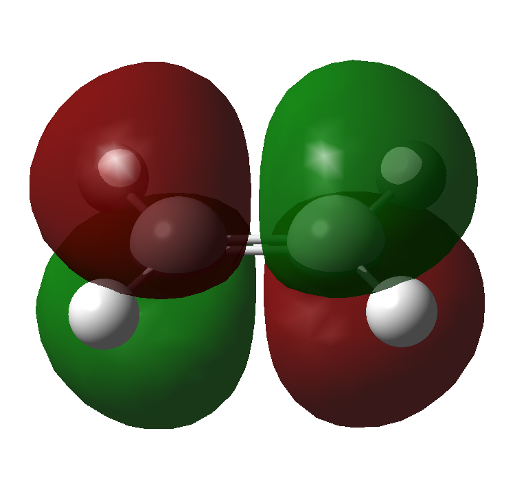
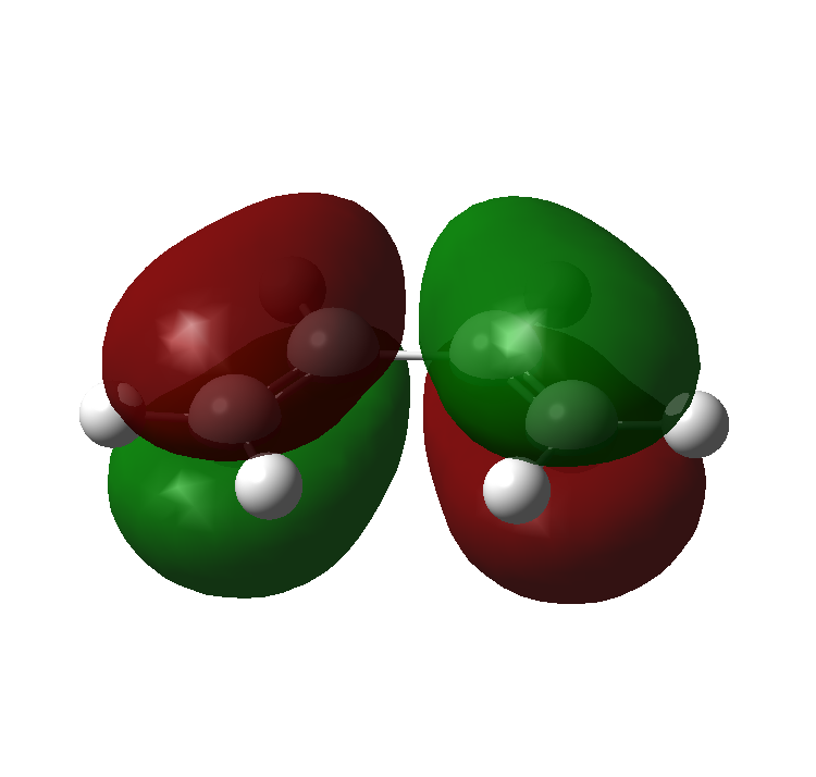
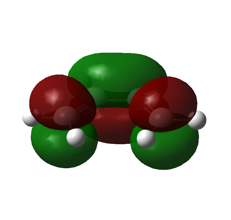
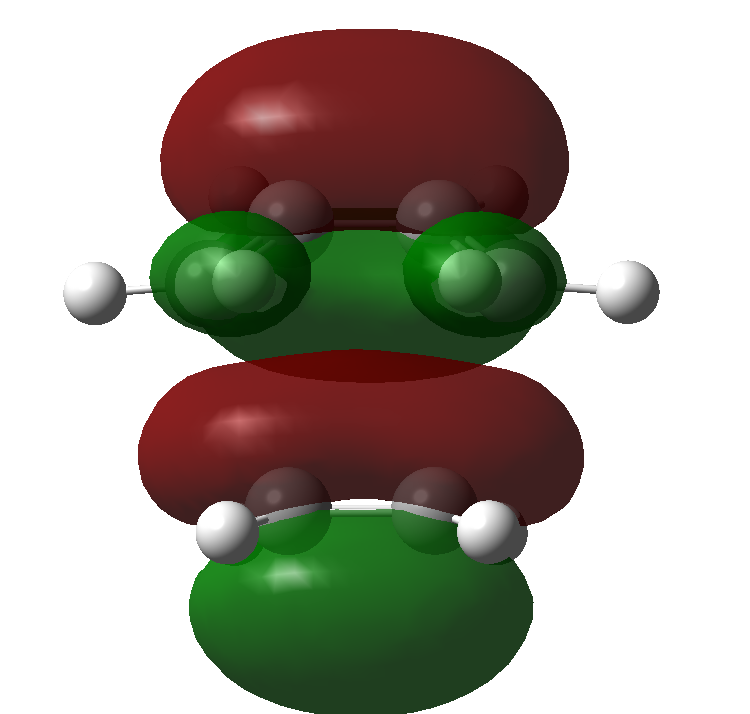
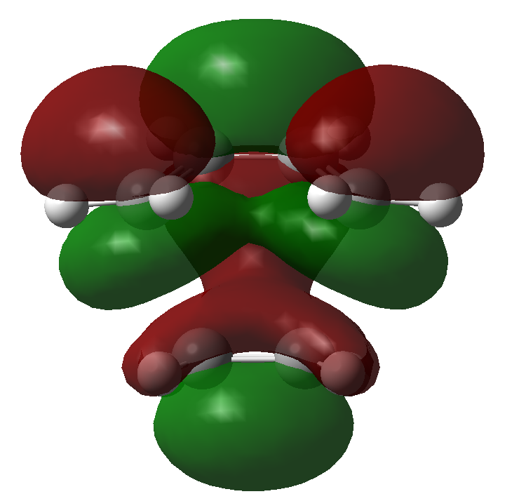
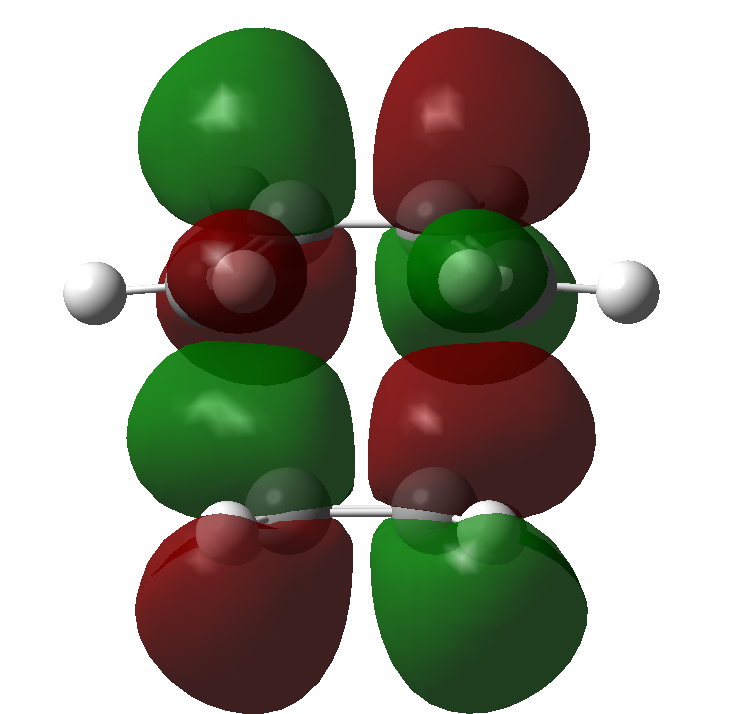
The molecular orbitals for ethene and butadiene calculated using Gaussian, with a Semi-empirical method and an AM1 forcefield can be seen here:
Ethene: HOMO, LUMO
Butadiene: HOMO, LUMO
The laws of quantum mechanics dictate that only orbitals of the same symmetry can interact and therefore there are only two interactions of the frontier molecular orbitals that can really take place. Either the HOMO of the diene and the LUMO of the dienophile or the LUMO of the diene and the HOMO of the dienophile. From the MO diagram in Scheme 15 we can see that the only interaction that is likely to occur is that between the HOMO of the diene and the LUMO of the dienophile because they are the closest match in energy.
In practice the reaction between butadiene and ethene to form cyclohexene is incredibly slow and can only be forced to take place at 165oC and 900atm for 17hr - giving a meagre 78% yield [5]. The reason why the simplest Diels-Alder reaction doesn't occur readily is twofold: firstly 1,5-butadiene does not exist for long in the higher energy s-cis conformation, and secondly because ethene is fairly electron rich, its LUMO does not match well to the HOMO of the diene. It is however, the simplest Diels-Alder reaction that can occur and hence a good starting point for analysis.
Transition state analysis of the Diels-Alder reaction between butadiene and ethene
As always we must first optimise the two reactants in the Diels-Alder reaction, ethene and s-cis-1,5-butadiene. The optimisation of these rather trivial structures was completed using a Semi-empirical method with an AM1 forcefield. Once the structures have been optimised a suitable method for the prediction of the likely TS structure can be chosen. From the three different methods that we have employed so far: directly calculating the force constant matrix, the frozen co-ordinate method and the QST2 method I have opted to calculate the force constant matrix directly. As previously discussed this method can be very time consuming and if the original guess is too far removed from a reasonable transition state the calculation will not work, I feel however that it does deliver a very accurate TS structure.
To calculate the transition state in this way we need to import our two optimised reactant structures into a single Gaussian calculation window. Once a reasonable guess as to the likely transition state had been made (terminal alkene carbons 2.1Å apart) taking into account the necessary orbital overlaps, the optimisation and frequency calculation was made to a Berny TS at the HF/3-21G level. The results are best visualised by the vibration of the transition state seen (here). The frequency of this imaginary vibration occurs at -818.35cm-1 and the equilibrium distance between the two terminal carbons is 2.21Å. The calculation was repeated again but this time using a more complex DFT method and large 6-31G(d) basis set. The frequency of this imaginary vibration occurs at -524.74cm-1 and the equilibrium distance between the two terminal carbons is 2.27Å, the vibration of the transition state seen (here). The results are shown in Scheme 16.
| Optimised TS(Berny) HF/3-21G | Optimised TS(Berny) B3LYP/6-31G(d) | ||||||
| Structure |
| ||||||
| Frequency of vibration (cm-1) | -818.35 | -524.74 | |||||
| Equilibrium C-C distance (Å) | 2.21 | 2.27 |
The results of the TS optimsiation in both cases gave only one imaginary vibration, indicating that a suitable transition state minima had been located. The nature of the imaginary vibrations are very important in determining what type of reaction the Diels-Alder actually is. Pericyclic reactions are specific category of reactions by which the transition state is cyclic and the proceeds in a concerted fashion. Put simply this means that there are no distinct high energy bond forming and breaking intermediates. The energy profile diagram for a pericyclic reaction is smooth and this is what is displayed by the vibrations. The movement of the butadiene towards the ethene and subsequent bond formation is synchronous and the two bonds form at the same time. The first few real vibrations show a distinct asynchronous movement of the orbitals towards each other therefore implying the reaction proceeding through a concerted transition state and hence an intermediate. These can be seen (here) for the HF/3-21G optimised TS occurring at 284.46cm-1, and (here) for the B3LYP/6-31G(d) optimised TS occuring at 203.90cm-1.
Intrinsic Reaction Co-ordinate method calculations
In order however to generate an overall picture of the transition state we need to perform an IRC calculation as before. The IRC allows us to see how the structure changes from the reactants through the transition state and to the product. Similarly to the IRC of the cope rearrangement we are going to calculate the force constants at every stage instead of once to ensure that the lowest energy conformation of the product and reactants are reached. The calculation was performed at the HF/3-21G level and the resulting Energy vs. Reaction co-ordinate graph can be seen in Scheme 17.

The corresponding RMS gradient graph can be seen (here). The IRC graph shown in Scheme 17 is typical of the energy profile diagram we would expect to see for a pericyclic reaction, a smooth transition state without any high energy intermediates. The IRC calculation was completed in 89 steps and the transition energy can be calculated from the data points (seen (here)) and the results are shown in Scheme 18.
| Number of reference points | ΔEActivation (kcal/mol) | ΔHReaction (kcal/mol) | TS Ethene C-C bond length (Å) | TS Butadiene C-C σ and C=C π bond lengths (Å) |
| 89 | 34.34 [lit. 27.5±2 (high temp)][6] | -39.17 | 1.38 [lit. 1.33][7] | σ - 1.39 [lit. 1.45], π - 1.37 [lit. 1.34][8] |
From the comparison of the theoretical values to the experimental values shown in Scheme 18 we can infer some important points about the transition state of the Diels Alder reaction. The large difference between the experimental and calculated activation energy is two fold, firstly the calculation was completed at the HF/3-21G level of theory for simplicity and speed, in reality this is poor representation of the true energy as it does not take into account electron correlations between orbitals. Secondly, it is not uncommon for calculated TS energies to be higher in energy than the experimental because it has to take into account the zero-point energy and other thermal energies and enthalpies. In addition to this the temperature at which the experimental was carried out is significantly larger than the temperature at which the calculation was carried out. Comparing the bond lengths of the transition state molecule to literature values of the bond lengths of 1,3-butadiene and ethene reveals a great deal about the structure of the molecules at the transition state. The ethene bond length is significantly shorter than the normal ethene bond length because this bond goes from a double to a single bond in the course of the reaction. We would expect that at the transition state it would be somewhere in between the normal values for a double and single bond. The two π bonds in butadiene are again shorter than the normal butadiene values because these two bonds form single bonds in the product, on the other hand the butadiene single bond is shorter than the normal value because this bond is going from single to double in character. The bond-length argument is compelling in arguing the case for a cyclic conjugated transition state like that described in Scheme 14.

Unfortunately the product cyclohexene as predicted by the IRC does not adopt the usual half chair conformation. Instead the cyclohexene produced is adopting a higher energy boat conformation (the transition conformer between the half chairs). This again highlights certain flaws in the method used to calculate the IRC using the HF/3-21G level of theory. The conformation of the cyclohexene product can be seen here.
An animation of the full IRC method can be seen (here) although the first few frames have been removed so the file could be uploaded.
Molecular orbitals at the Transition state
There are certain conditions outlined about pericyclic reactions published by Woodward and Hoffmann in 1965[9] that state for a thermal [4+2] cycloaddition such as the Diels-Alder reaction, the two components must react suprafacially. This means that the diene must attack only one face of dienophile (or vice versa) (Scheme 19). From Scheme 15 we can see that the Diels-Alder reaction occurs by the interaction of the HOMO of the diene and the LUMO of the dienophile, as one can see from Scheme 19 these can interact in two different ways, either suprafacially or antarafacially. As we have already discussed however, under the conditions set out, the diene and the dienophile are only allowed to react suprafacially. The fact that two anti-symmetric orbitals are interacting suprafacially the resulting transition state molecular orbitals should be symmetric. The transition state molecular orbitals calculated to the HF/3-21G level are shown below:
Transition State MOs: HOMO-1, HOMO, LUMO, LUMO+1
As we can see the HOMO and LUMO molecular orbitals lend themselves well to the computed reaction co-ordinte and possess the desired symmetry. A point to consider however is why the reaction does not take place at the LUMO of ethene and the HOMO of butadiene as they possess the correct symmetry and orbital overlap required to technically react. The answer lies in the energies of orbitals, the HOMO of ethene and LUMO of butadiene are very similar in energy and hence the overlap is very large. The LUMO of ethene and HOMO of butadiene are far removed from each other and hence the overlap is very small. It is however large enough to cause a small stabilisation of the transition state called inverse electron demand.
Diels Alder reaction of 1,3-Cyclohexadiene and Maleic anhydride
Introduction

Unlike the previous Diels Alder reaction between ethene and 1,3-butadiene which is far too sluggish to occur at room temperature and pressure, the reaction between 1,3-cyclohexadiene and maleic anhydride is several orders of magnitude better. Maleic anhydride is an incredibly electron deficient alkene due to the electron withdrawing effect of the two carbonyls, lowering the LUMO energy and cyclohexadiene is held permanently held in the s-cis conformation. Furthermore unlike the reaction between butadiene and ethene there are additional stereoselective considerations to take into account. In the reaction between ethene and butadiene it did not matter which way around the ethene added so long as it did so suprafacially however when the product contains a bridge there are two possible outcomes (Scheme 20). The terms endo- and exo- isomers come from the relative orientation of the diene and dienophile in the transition state. If the main body of the dienophile extends under the body of the diene in the transition state then the endo- isomer is produced, conversely if the main body of the diene points away from the dieneophile then the exo-product is produced. The normal distribution of products tends to greatly favour the formation of the endo- isomer which is considered to be the kinetic product. The thermodynamically favoured exo- isomer can be formed with prolonged reaction times and high temperatures. Kinetic reactions are often irreversible and the product formed is the one with the lowest barrier to formation, on the other hand thermodynamic reactions are reversible and over time the most thermodynamically stable product is formed. We are going to look at the relative energies of the two transition states and identify which pathway is preferred and why.
To start we need to optimise the two reactant molecules, 1,3-cyclohexadiene and maleic anhydride. We are going to use a Semi-empirical method with an AM1 basis set to optimise the structures and transition states throughout the exercise. The semi-empirical method is based on Hartree-Fock theory but makes more approximations based on a certain set of empirical parameters. Despite these approximations it is widely used in computational chemistry for its ability to analyse large molecules and transition states quickly and cheaply as well as providing results that fit experimental data well. The structures of the molecules were optimised and the MOs calculated at the Semi-empirical level/AM1 and the results are shown in Schemes 21 (Cyclohexadiene) and 22 (Maleic anhydride).


As we have seen in the Diels Alder reaction between ethene and butadiene, the frontier molecular orbitals posses the same symmetric and antisymmetric properties and the reaction takes place between the antisymmetric LUMO of maleic anhydride and the antisymmetric HOMO of cyclohexadiene.
Transition state analysis
Once the structures had been optimised the two transition states (exo- and endo-) could be optimised in the same manner as that used previously. Due to the relative complexity of the structures using the frozen co-ordinate method is the most appropriate method to use. As previously described the frozen co-ordinate method locks the position of the bonding atoms at a fixed distance while performing an optimisation on the rest of the molecule. Once the first optimisation is complete one can then unfreeze the co-ordinates of the bonds and differentiate along the path using a numerical hessian. This method is very cost-effective and doesn't require a so called lucky guess with the geometry of the input transition state. With the complexity of the molecules involved, the semi-empirical AM1 forcefield was invoked and the molecules calculated to a Berny TS and the results are shown in Scheme 23.
| Optimised Exo-TS(Berny) | Optimised Endo-TS(Berny) | ||||||
| Structure |
| ||||||
| Frequency of vibration (cm-1) | -812.26 | -806.73 | |||||
| Equilibrium C-C distance (Å) | 2.17 | 2.16 |
The Berny TS calculations both converged to a minimum successfully with one imaginary vibration each. An animation of the vibration for the exo- TS can be seen (here) and the endo- TS can be seen (here). These vibrations correspond satisfactorily to what the real bond formation should look like, with the synchronous formation of the both bonds. The first real vibrations of the molecules is a twisting motion which corresponds to an asynchronous type formation of the two molecules, the animations for the first real vibration at 60.87cm-1 for the exo- TS can be seen (here) and for the endo- TS at 62.45cm-1 (here).
From the optimised transition states we can garner information about the bond lengths and how these compare to the equilibrium ground state values. The values of the bond lengths taken are taken from the highest energy TS conformation and the ground state values taken from the original optimised structures, both at the semi-empirical/AM1 level. The results are shown in Scheme 24.
| Diene C=C-C-C-C=C σ bond (Å) | Diene C=C π bond (Å) | Dienophile C=C π bond (Å) | |
| Exo- TS | 1.40 | 1.40 | 1.41 |
| Endo- TS | 1.40 | 1.40 | 1.41 |
| Optimised GS Structure | 1.45 | 1.34 | 1.35 |
From Scheme 24 we can see that the optimised GS bond lengths vary considerably with the TS bond lengths, which is to be expected. The TS state bond lengths for the both the exo- and endo- are the same to 2 d.p. which is of little surprise and neither is the fact that the σ and π bond lengths are so close. This really highlights the fact that this process occurs via a concerted mechanism in a cyclic transition state. This is reinforced by comparing the TS values to the optimised GS values where we see that as the π bonds turn into σ bonds their bond length is intermediate between the two and the reverse is true for the σ to π bond.
Intrinsic Reaction Co-ordinate Calculations
Once the transition state structures have been identified we can run an IRC calculation tracking the energy of the structures from reactants to products. The force constants were calculated at every step and at the semi-empirical/AM1 level. The IRC was run in both directions with a maximum number of co-ordinates 150 to ensure the optimisations ran to completion. The energy vs. reaction co-ordinate graphs for the exo- and endo- reactions are shown in Schemes 25 with the activation energy and enthalpy of reaction added. (Note: The exo- TS IRC calculation ran backwards (ie. product to reactant) and so the reaction co-ordinate appears backwards and has accordingly been inverted in the graph)
| Exo product | Endo product | |||||
 |
 | |||||
|
The exo- IRC calculation was completed in 93 steps with the highest energy TS found at step 25 (N.B. product to reactant), the individual energies can be found (here) as well as the RMS gradient graph (here). The endo- IRC calculation was completed in 100 steps with the highest energy TS found at step 74, the individual energies can be found (here) as well as the RMS gradient graph (here).
A movie showing the full reaction co-ordinate can be can be seen here: Exo and Endo
From Scheme 26 we can clearly see that the activation barrier for the endo- product is lower than the exo- indicating that the endo- product is the kinetic product of the reaction. What is more interesting are the relative reaction enthalpies. As we discussed in the introduction the exo- product is usually the thermodynamic product however from the calculation results the endo- product seems to be both kinetically and thermodynamically favoured. This result is confirmed by an MM2 energy optimisation calculation (performed in ChemBioUltra 3D) (endo-35.1425kcal/mol, exo-36.5685kcal/mol). What is clear is that the energy difference between the two products is very small and perhaps needs a higher degree of electron correlation in the calculation to give an accurate result (DFT).
Molecular orbital interactions at the transition state
It has been shown that the principal orbital interaction that drives the Diels Alder reaction occurs between the HOMO of cyclohexadiene and the LUMO of maleic anhydride. These two orbitals combine as they are similar in energy thanks to the electron withdrawing effect of the carbonyls lowering the relative energy of the LUMO. The combination of two antisymmetric orbitals leads to a new set of antisymmetric orbitals as shown in Schemes 26 and 27 for the endo- and exo- transition states (at the semi-empirical/AM1 level).
| Orbital | HOMO-1 | HOMO | LUMO | LUMO+1 |
| Structure |  |
 |
 |
 |
| Relative energy | -0.3684 | -0.3451 | -0.0357 | -0.0201 |
| Symmetry | Symmetric | Antisymmetric | Symmetric | Antisymmetric |
| Orbital | HOMO-1 | HOMO | LUMO | LUMO+1 |
| Structure |  |
 |
 |
 |
| Relative energy | -0.3667 | -0.3428 | -0.0405 | -0.0201 |
| Symmetry | Symmetric | Antisymmetric | Symmetric | Antisymmetric |

The same symmetry pattern is observed in the exo- and endo-transition state with a nodal plane down the centre of the two molecules in the HOMO and LUMO, bisecting the O=C-O-C=O of the maleic anhydride. The reason why the endo- TS preferred over the exo- puzzled scientists for many years because from a pure steric standpoint it shouldn't, the resulting endo- product is a more strained ring. It wasn't until Woodward, Hoffmann and Fukui suggested an orbital phenomenon known as secondary orbital overlap that it was explained. In the endo- transition state the non-bond forming π orbitals in the diene HOMO interact with the carbonyl π* orbitals of the dienophile LUMO, stabilising the system (Scheme 28). This effect is obviously not possible in the exo- transition state as the diene and dienophile bodies are orientated away from each other. The secondary orbital overlap can be visualised in the LUMO+1 of the endo- TS which is not expected. The strange ordering of the orbitals may be as a result of insufficient depth in the calculation, taking into account the primitive nature of the semi-empircal method. Calculating the orbitals at the HF or DFT level may well improve the accuracy of the ordering of the orbitals. The large nodal plane is no doubt as a result of the electron withdrawing carbonyls reducing the size of the π cloud in the HOMO but increasing the size of the π* interactions in the LUMO.
One factor that still needs addressing is the thermodynamic stability of the endo- and exo-products. It is clear from the empirical evidence and thermodynamic properties that the endo- product is kinetically favoured due to the secondary orbital overlap (Scheme 29) however what is not clear is why it is apparently favoured thermodynamically as well. We know that given time the less strained ring exo- product (thermodynamically most stable) will form where the bulky substituent lies in an equatorial plane. The only conclusion that can be drawn from this is that the level of calculation is not sufficient to take into account these factors.
Conclusion
During these exercises we have seen that is is possible to model the transition states of simple reactions. This tool is immensely powerful in initially predicting whether reactions are likely to occur or not before going into a lab and potentially waste time and money. Most reactions produce a mixture of isomers which can be very frustrating for the chemist to analyse and separate. Thermodynamic properties of the products and reactants allow us to make predictions about the formation of certain isomers over others by calculating activation energies in the transition state. One thing that we have seen however is that these calculations are not always accurate. Like the chemistry that occurs in the test tube, we can not always predict the correct outcome because other factors beyond the scope of the calculation come into effect. We have used three methods of calculation in this assignment, the Semi-empirical method, the Hartree-Fock method and the Density-Function method all with a variety of basis sets. The methods and basis sets used are only a very small portion of the techniques available to the computational chemist however as the method and basis set become more complex so the cost and time taken increase. For small molecules and simple reactions like the ones that have been performed here, the methods and basis sets do not need to be large and complex. For much larger reactions and molecules however a more rigorous level of calculation needs to be employed in order to get a sensible and reliable result.
Technical notes
All calculations unless otherwise stated were carried out using either Gaussian03 or Gaussian09 and the results visualised in GaussView 5.0. All molecules were constructed in GaussView 5.0 and optimised using either the Semi-empirical method with an AM1 forcefield, the Hartree-Fock method with a 3-21G basis set or the DFT method with a 6-31G(d) basis set. IRC calculations were completed with force constants calculated at every point unless otherwise stated. All QST2 TS optimisations were completed without calculating the force constants.
The conversion was used throughout:
1Ha = 627.5095 kcal/mol
Appendix
A selection of Gaussian Output files have been ordered by section if further investigation is needed. If any file is not present here it is available upon request:
HF=Optimised to the HF/3-21G level, DFT=Optimised to the DFT/B3LYP/6-31G(d) level and AM1=Optimised to the Semi-empirical/AM1 level
1,5-hexadiene conformations optimisations: Anti-2 HF, Anti-2 DFT, Anti-1 HF, Gauche-3 HF
Anti-2 conformation Opt+Freq: Anti-2 DFT 0K, Anti-2 DFT 1K, Anti-2 DFT 521.15K
Chair TS(Berny): Chair TS(Berny) HF, Chair TS(Berny) DFT
Allyl fragment: Allyl fragment HF
Chair TS frozen Co-ordinate: Chair TS Frozen Co-ordinate HF, Chair TS Frozen Co-ordinate DFT
Boat TS QST2: Boat TS QST2 HF, Boat TS QST2 DFT
Chair TS IRC: Chair TS IRC HF
1,3-Butadiene optimisation: 1,3-Butadiene AM1
Ethene optimisation: Ethene AM1
Diels Alder TS optimisation: Diels Alder TS HF, Diels Alder TS DFT
Diels Alder IRC: Diels Alder IRC HF
1,3-Cyclohexadiene optimisation: 1,3-Cyclohexadiene AM1
Maleic anhydride optimisation: Maleic anhydride AM1
Exo TS optimisation: Exo TS AM1
Exo TS IRC: Exo IRC AM1
Endo TS optimisation: Endo TS AM1
Endo TS IRC: Endo IRC AM1
References
- ↑ Nishio,M.;Hirota,M. Tetrahedron, 1989, 45 , 7201
- ↑ BRANDON G. ROCQUE, JASON M. GONZALES & HENRY F. SCHAEFER III (2002): An analysis of the conformers of 1,5- hexadiene, Molecular Physics: An International Journal at the Interface Between Chemistry and Physics, 100:4, 441-446
- ↑ J. Am. Chem. Soc., 1994, 116 (22), pp 10336–10337
- ↑ https://wiki.ch.ic.ac.uk/wiki/index.php?title=Mod:phys3#Results_Table
- ↑ Fleming, Ian. Pericyclic reactions: Oxford Chemistry Primer 67, 1998, page 7
- ↑ J. Phys. Chem. A, 2001, 105 (43), pp 9945–9953
- ↑ J Phys Chem A. 2006 Jun 15;110(23):7461-9.
- ↑ J Phys Chem A. 2006 Jun 15;110(23):7461-9.
- ↑ J. Am. Chem. Soc.; 1965; 87(2); 395-397. doi:10.1021/ja01080a054