Y3C Monte-Carlo simulations of a 2D Ising Model

Task 1

TASK: Show that the lowest possible energy for the Ising model is
$E = - D N J$
, where
$D$
is the number of dimensions and
$N$
is the total number of spins. What is the multiplicity of this state? Calculate its entropy.

For the lowest possible energy, all the spins must be aligned. Hence, the $s_{i} s_{j}$ term is always positive and has a value of 1 for each neighbours. Since this is the case, the expression $\sum_{j \in n e i g h b o u r s (i)} s_{i} s_{j}$ can be expressed in terms of the dimensions. For each dimension $D$ , the expression becomes $2 D$ . $\sum_{i}^{N}$ now becomes the number of molecules $N$ . Combining all the expressions, the energy simplifies to $E = - D N J$ . Since all the spins are align, there are only 2 configurations. One where all the spins are aligned up and one down. Therefore, the entropy would be $9.57 \times 1 0^{- 24}$ (as $S = k l n W$ ).

Task 2

TASK: Imagine that the system is in the lowest energy configuration. To move to a different state, one of the spins must spontaneously change direction ("flip"). What is the change in energy if this happens (
$D = 3, N = 1000$
)? How much entropy does the system gain by doing so?

The change in the energy would be $+ 6 J$ as there will be six neighbours to the flipped spin that has different spin state. Using combinatorics, the number of permutations $(W)$ for this state is $W = 2 \times (\frac{1000!}{1! \times 999!}) = 2000$ . Hence, as $S = k l n W$ , the entropy gained by this would be $1.05 \times 1 0^{- 22} J K^{- 1}$ .

Task 3

TASK: Calculate the magnetisation of the 1D and 2D lattices in figure 1. What magnetisation would you expect to observe for an Ising lattice with
$D = 3, N = 1000$
at absolute zero?

For the calculations in figure 1:

$M = + 1$ (for 1D)

$M = + 1$ (for 2D)

As Gibbs free energy of the system is $Δ G = Δ H + T Δ S$ , at absolute zero, entropy has no contribution to the total Gibbs energy. Hence as now $Δ G = Δ H$ , the configuration that has the lowest Gibbs energy is when all the spins are aligned (Third Law of Thermodynamics) as this has the lowest free energy (most stable). Therefore, the total magnetisation must be $\pm 1000$ . Note that the two magnetization states are degenerate.

Task 4

TASK: complete the functions energy() and magnetisation(), which should return the energy of the lattice and the total magnetisation, respectively. In the energy() function you may assume that
$J = 1.0$
at all times (in fact, we are working in reduced units in which
$J = k_{B}$
, but there will be more information about this in later sections). Do not worry about the efficiency of the code at the moment — we will address the speed in a later part of the experiment.

def energy(self):
       "Return the total energy of the current lattice configuration."
       energy = 0.0
       "horizontal interactions was calculated here"
       e11 = 0
       for i in list(range(len(self.lattice))):
           e12 = 0
           for j in list(range(len(self.lattice[i]))):
               if j is list(range(len(self.lattice[i])))[0]:
                   e12 = e12 + (self.lattice[i,j]*self.lattice[i,-1]) + (self.lattice[i,j]*self.lattice[i,j+1])
               elif j is list(range(len(self.lattice[i])))[-1]:
                   e12 = e12 + (self.lattice[i,j]*self.lattice[i,0]) + (self.lattice[i,j]*self.lattice[i,j-1])
               else:
                   e12 = e12 + (self.lattice[i,j]*self.lattice[i,j+1]) + (self.lattice[i,j]*self.lattice[i,j-1])
           e11 = e11 + e12
       
       "vertical interactions here"
       e21 = 0
       for k in list(range(len(self.lattice))):
           e22 = 0
           for l in list(range(len(self.lattice[k]))):
               
               if k is list(range(len(self.lattice[k])))[0]:
                   e22 = e22 + (self.lattice[k,l]*self.lattice[-1,l]) + (self.lattice[k,l]*self.lattice[k+1,l])
               elif k is list(range(len(self.lattice[k])))[-1]:
                   e22 = e22 + (self.lattice[k,l]*self.lattice[0,l]) + (self.lattice[k,l]*self.lattice[k-1,l])
               else:
                   e22 = e22 + (self.lattice[k,l]*self.lattice[k+1,l]) + (self.lattice[k,l]*self.lattice[k-1,l])
           e21 = e21 + e22
               
       energy = (e21+e11)*(-1/2)
       return energy

   def magnetisation(self):
       "Return the total magnetisation of the current lattice configuration."
       mag_moment1 = 0
       for i in list(range(len(self.lattice))):
           mag_moment1 = mag_moment1 + self.lattice[i]
       magnetisation = 0
       for j in list(range(len(mag_moment1))):
           magnetisation = magnetisation + mag_moment1[j]
       return magnetisation

Task 5

TASK: Run the ILcheck.py script from the IPython Qt console using the command
%run ILcheck.py
The displayed window has a series of control buttons in the bottom left, one of which will allow you to export the figure as a PNG image. Save an image of the ILcheck.py output, and include it in your report.

Task 6

TASK: How many configurations are available to a system with 100 spins? To evaluate these expressions, we have to calculate the energy and magnetisation for each of these configurations, then perform the sum. Let's be very, very, generous, and say that we can analyse
$1 \times 1 0^{9}$
configurations per second with our computer. How long will it take to evaluate a single value of
${⟨ M ⟩}_{T}$
?

The number of different configurations/states is $S = 2^{100} = 1.27 \times 1 0^{30}$ . It would take $4.02 \times 1 0^{13} y e a r s$ !

Task 7

TASK: Implement a single cycle of the above algorithm in the montecarlocycle(T) function. This function should return the energy of your lattice and the magnetisation at the end of the cycle. You may assume that the energy returned by your energy() function is in units of
$k_{B}$
! Complete the statistics() function. This should return the following quantities whenever it is called:
$< E >, < E^{2} >, < M >, < M^{2} >$
, and the number of Monte Carlo steps that have elapsed.

   def montecarlostep(self, T):
       
       energy = self.energy()
       random_i = np.random.choice(range(0, self.n_rows))
       random_j = np.random.choice(range(0, self.n_cols))
       
       random_number = np.random.random()
               
       if self.lattice[random_i,random_j] == 1:
           self.lattice[random_i,random_j] = -1
       else:
           self.lattice[random_i,random_j] = 1

       dE = self.energy() - energy
       if dE <= 0:
           energy = self.energy()  
       elif random_number <= np.exp((-dE)/(T)):
           energy = self.energy()
       else:
           if self.lattice[random_i,random_j] == 1:
               self.lattice[random_i,random_j] = -1
           else:
               self.lattice[random_i,random_j] = 1
       
       
       self.E += self.energy()
       self.E2 += self.energy()**2
       self.M += self.magnetisation()
       self.M2 += self.magnetisation()**2
       self.n_cycles +=1
       energy = self.energy()
       magnetisation = self.magnetisation()
       
       return energy,magnetisation

   def statistics(self):
       # complete this function so that it calculates the correct values for the averages of E, E*E (E2), M, M*M (M2), and returns them
       self.E_ = self.E/self.n_cycles
       self.E2_ = self.E2/self.n_cycles
       self.M_= self.M/self.n_cycles
       self.M2_ = self.M2/self.n_cycles
       
       return self.E_,self.E2_, self.M_, self.M2_

Please see the comments at the end of the wiki page at the source code section.

Task 8

TASK: If
$T < T_{C}$
, do you expect a spontaneous magnetisation (i.e. do you expect
$⟨ M ⟩ \neq 0$
)? When the state of the simulation appears to stop changing (when you have reached an equilibrium state), use the controls to export the output to PNG and attach this to your report. You should also include the output from your statistics() function.

From the simulation carried out, when $T < T_{C}$ at equilibrium, all the spins are aligned. when the temperature is less than the Curie temperature, magnetization will be spontaneous. Essentially, this is because the enthalpy term dominates due to low temperature. After $T_{C}$ , the entropic term dominates and magnetization now will not be spontaneous. At temperature larger than the Curie temperature, it would require energy to align all the spins to be parallel (eg. apply external field).

Task 9

TASK: Use the script ILtimetrial.py to record how long your current version of IsingLattice.py takes to perform 2000 Monte Carlo steps. This will vary, depending on what else the computer happens to be doing, so perform repeats and report the error in your average!

The average time for my computer is $32.559503 \pm 0.536841202 s e c o n d s$ .

Task 10

TASK: Look at the documentation for the NumPy sum function. You should be able to modify your magnetisation() function so that it uses this to evaluate M. The energy is a little trickier. Familiarise yourself with the NumPy roll and multiply functions, and use these to replace your energy double loop (you will need to call roll and multiply twice!).

For the energy calculation, the np.roll function was called twice as suggested to calculated the interactions in the horizontal and the vertical orientation. After that, the np.multiply and the np.sum was used to calculated the resulting energy.

   def energy(self):
       "Return the total energy of the current lattice configuration."
       return (-1)*(np.sum((np.multiply(self.lattice, np.roll(self.lattice,1,axis=0))
                    +np.multiply(self.lattice,np.roll(self.lattice,1,axis=1)))))

As for the magnetization, I simply used the np.sum to calculate the total magnetization.

   def magnetisation(self):
       "Return the total magnetisation of the current lattice configuration."
       return np.sum(self.lattice)

Task 11

TASK: Use the script ILtimetrial.py to record how long your new version of IsingLattice.py takes to perform 2000 Monte Carlo steps. This will vary, depending on what else the computer happens to be doing, so perform repeats and report the error in your average!

The average time for the new quote is $0.440910375 \pm 0.015088522 s e c o n d s$

Task 12

TASK: The script ILfinalframe.py runs for a given number of cycles at a given temperature, then plots a depiction of the final lattice state as well as graphs of the energy and magnetisation as a function of cycle number. This is much quicker than animating every frame! Experiment with different temperature and lattice sizes. How many cycles are typically needed for the system to go from its random starting position to the equilibrium state? Modify your statistics() and montecarlostep() functions so that the first N cycles of the simulation are ignored when calculating the averages. You should state in your report what period you chose to ignore, and include graphs from ILfinalframe.py to illustrate your motivation in choosing this figure.

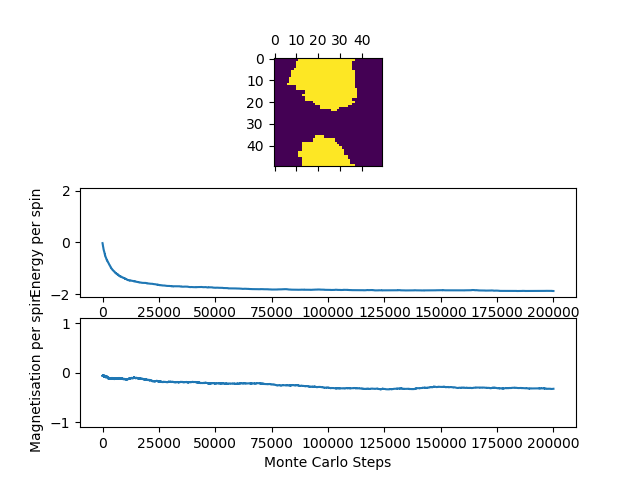
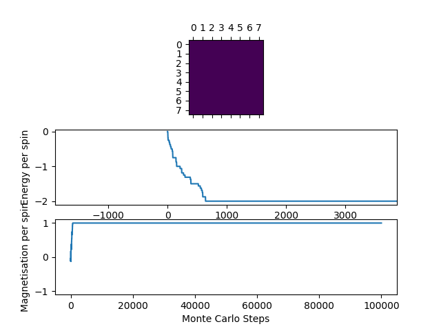
In general, the lower the temperature and the bigger the lattice size requires more time to reach equilibrium. Assuming the upper most limit is $50 \times 50$ at $T = 1$ (see below), it takes around $100, 000$ cycles to reach the equilibrium. In fact, for the run below (first plot), the system has reached a 'metastable' state where approximately half of the spins are up and half are down (evident from the magnetization per spin), with aligned spins forming large clusters. This was found to be common for systems at lower temperature (well below the Curie temperature). As a result, this had affected the calculations and analysis in the later sections.

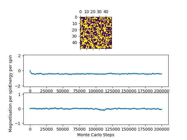
Just to show how the temperature affects the amount of cycles it takes to reach equilibrium, the ILfinalframe was ran for 50 by 50 lattice at $T = 5$ (see below).

Hence, to make sure that all the rest of the runs reach equilibrium before taking the average values, I would start taking the average after $100, 000$ cycles.

Actually, it was found later in the next tasks that it is best to modify the IsingLattice and the ILtemperature for different lattice systems before running the script, as this saves lots of time. For instance, for the $2 \times 2$ case, it takes less than 1000 cycles to reach equilibrium. Whereas for the $32 \times 32$ case at $T = 0.25$ , it can take more than 200,000 cycles to reach equilibrium.

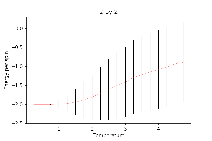
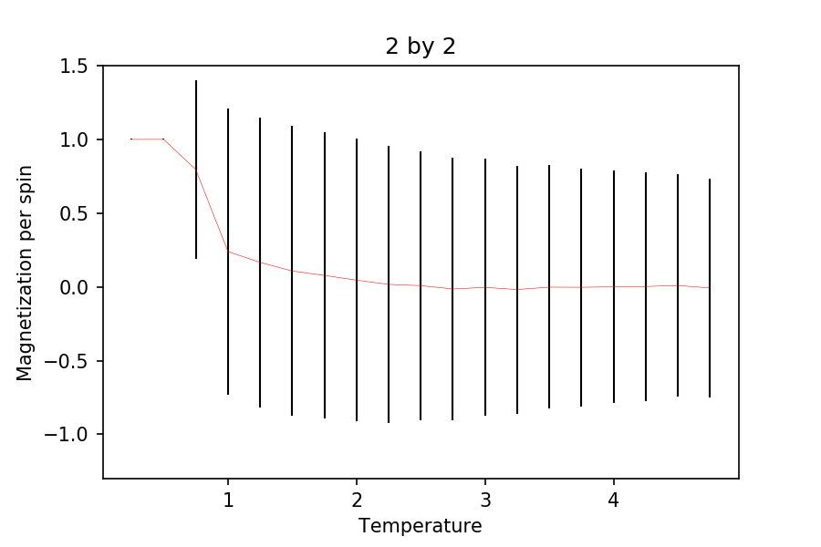
It was also found that for the 2 by 2 case, the energy fluctuates enormously when a spin is flipped. This is because there are only 4 spins in total, which means the energy change in flipping a spin is similar to the total energy overall. The same goes for the magnetization of the system.

Task 13

TASK: Use ILtemperaturerange.py to plot the average energy and magnetisation for each temperature, with error bars, for an
$8 \times 8$
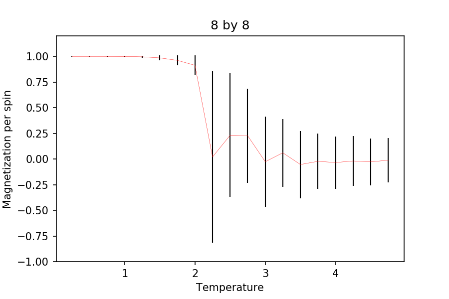
lattice. Use your initution and results from the script ILfinalframe.py to estimate how many cycles each simulation should be. The temperature range 0.25 to 5.0 is sufficient. Use as many temperature points as you feel necessary to illustrate the trend, but do not use a temperature spacing larger than 0.5. T NumPy function savetxt() stores your array of output data on disk — you will need it later. Save the file as 8x8.dat so that you know which lattice size it came from.

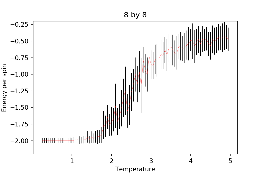
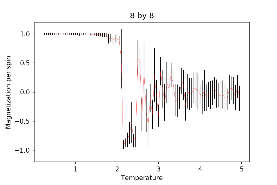
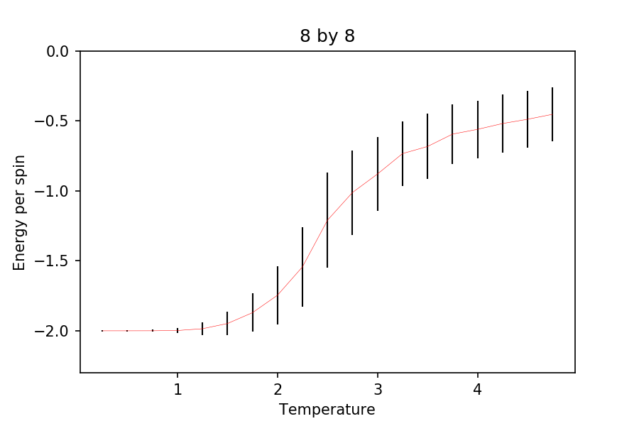
From running the ILfinalframe on different systems, I think it would take around $5000$ n cycles to reach equilibrium. In fact, it takes around 700 n cycles to reach equilibrium due to its small size, despite the lower temperature (ILfinalframe ran at 8 by 8 at $T = 0.25$ . Although, to make sure that all the different states equilibrate, 3000 cycles were ran before the calculated energy and magnetization were collected and average/standard deviation calculated. Note that a further 3000 cycles were ran, so the total cycles used for each temperature is 6000.

And below is the Energy/Magnetization per spin against Temperature plot obtained from running ILtemperaturerange.

The temperature used was between 0.25 and 5, increasing by 0.05.

Task 14

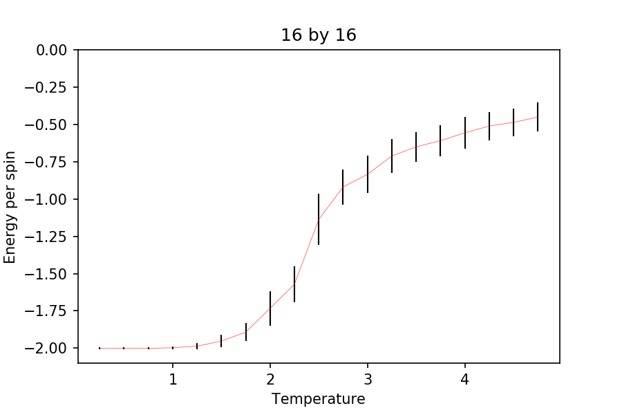
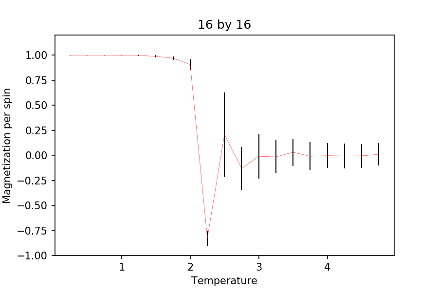
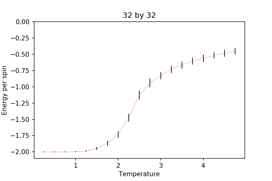
TASK: Repeat the final task of the previous section for the following lattice sizes: 2x2, 4x4, 8x8, 16x16, 32x32. Make sure that you name each datafile that your produce after the corresponding lattice size! Write a Python script to make a plot showing the energy per spin versus temperature for each of your lattice sizes. Hint: the NumPy loadtxt function is the reverse of the savetxt function, and can be used to read your previously saved files into the script. Repeat this for the magnetisation. As before, use the plot controls to save your a PNG image of your plot and attach this to the report. How big a lattice do you think is big enough to capture the long range fluctuations?

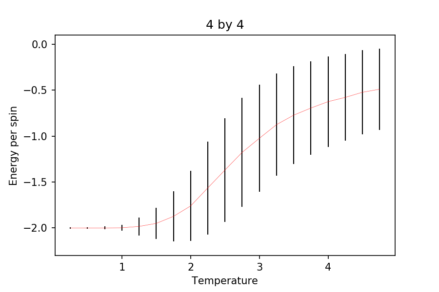
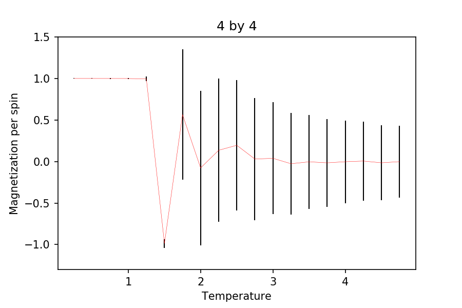
Again, ILfinalframe was used to check how many cycles it takes for the $32 \times 32$ system to reach equilibrium. It turns out that it takes roughly around 100,000 cycles to reach equilibrium. Hence, the first 250,000 cycles were not used for averaging and only the 150,000 steps after were used. Also, the ILfinalframe were carried out at $T = 0.25$ (upper limit for the number of cycles before reaching equilibrium). This is to make sure that all the energies and magnetizations are at their equilibrium state. Note that 7 repeats were carried out for each simulations. The temperature used was between 0.25 and 5, increasing by 0.25.

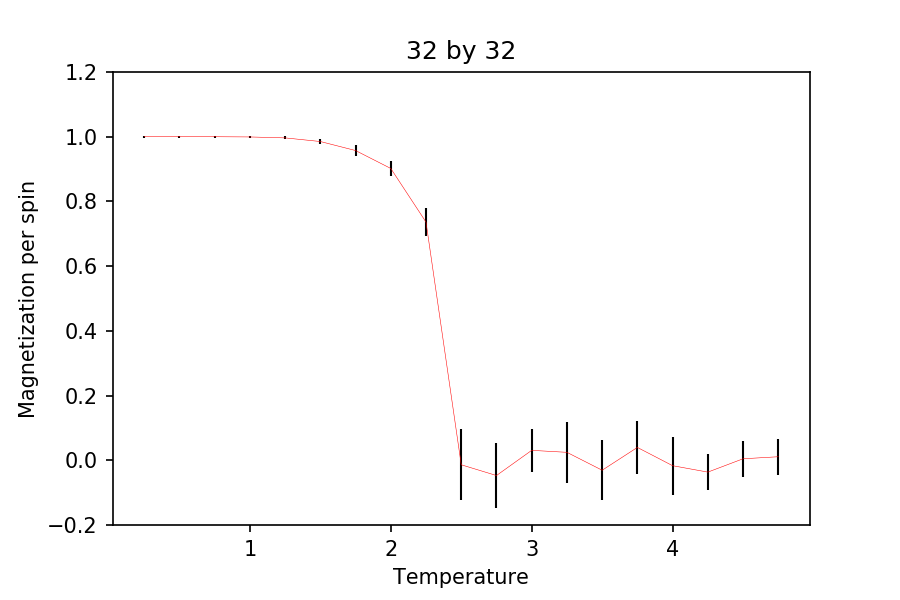
It can be seen that as the lattice size increases, the standard deviation of the energies and the magnetizations decreases quite rapidly. Also, it can be seen that the energy plots become more pronounced as the lattice size is increased. Although, there is not much difference from $L = 16$ onwards. The steep gradient and the change in magnetization (without external field) suggests phase transition but is not clear enough to indicate that it is the case (see later sections for this). At the very low temperature, it is expected that the energy per spin is $- 2$ , as this indicates that all the spins are aligned parallel (expected when $T < T_{C}$ , where $E / N = - 2$ .

As for the magnetization plots, it can be seen that as the lattice size increases, the change in the magnetization becomes more pronounced. Again, after $L = 16$ , the change in the plots becomes very small and indistinguishable to the larger lattices. At low temperature, it can be seen that all the spins are aligned parallel (agreed with theory).

From this, a lattice of 50 by 50 should be enough to capture the long range fluctuations, as after $16 \times 16$ , the energy and the magnetization plot doesn't change much at all. Note that the number of temperature range used here is less than that of the simulations ran before in the previous section. This is to save time as it can take a very long time to run such simulations for bigger lattices, as they require more cycles to reach equilibrium. In addition, the results obtained were very noisy and the analysis carried out afterwards were not of good quality compared to literature and the C++ data given. Hence, it was concluded that this condition gave the best results.

Task 15

TASK: By definition,
$C = \frac{\partial ⟨ E ⟩}{\partial T}$
From this, show that
$C = \frac{V a r [E]}{k_{B} T^{2}}$
(Where
$V a r [E]$
is the variance in
$E$
.)

As the system we are using is based on the canonical ensemble, the mean energy is as follows:

$⟨ E ⟩ = \frac{1}{Z} \sum_{α} E (α) \exp {- \frac{E (α)}{k_{B} T}}$

Although, this can be rewritten in terms of the partition function, which is a nicer expression:

$⟨ E ⟩ = - \frac{\partial}{\partial β} l n Z$

We also know that variance is as follows:

$V a r [E] = ⟨ (Δ E)^{2} ⟩ = ⟨ (E - ⟨ E ⟩)^{2} ⟩$

This again can be rewritten as:

$V a r [E] = ⟨ (Δ E)^{2} ⟩ = \frac{\partial^{2} \ln Z}{\partial β^{2}} = - \frac{\partial ⟨ E ⟩}{\partial β}$

And since:

$⟨ E ⟩ = \frac{\partial}{\partial β} = - k T^{2} \frac{\partial}{\partial T}$

Hence,

$V a r [E] = - \frac{\partial ⟨ E ⟩}{\partial β} = k T^{2} \frac{\partial ⟨ E ⟩}{\partial T} = k T^{2} C$

Giving:

$C = \frac{V a r [E]}{k_{B} T^{2}}$

Task 16

TASK: Write a Python script to make a plot showing the heat capacity versus temperature for each of your lattice sizes from the previous section. You may need to do some research to recall the connection between the variance of a variable,
$V a r [X]$
, the mean of its square
$⟨ X^{2} ⟩$
, and its squared mean
${⟨ X ⟩}^{2}$
. You may find that the data around the peak is very noisy — this is normal, and is a result of being in the critical region. As before, use the plot controls to save your a PNG image of your plot and attach this to the report.

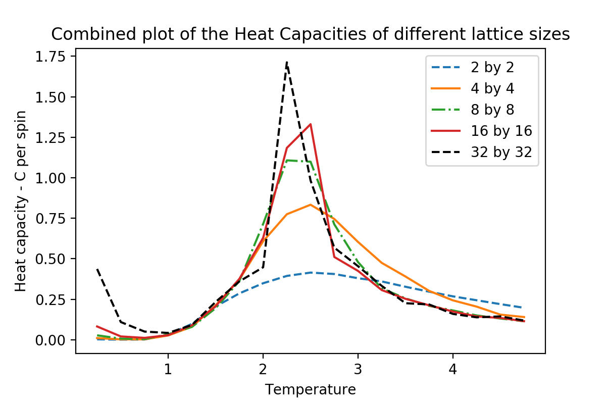
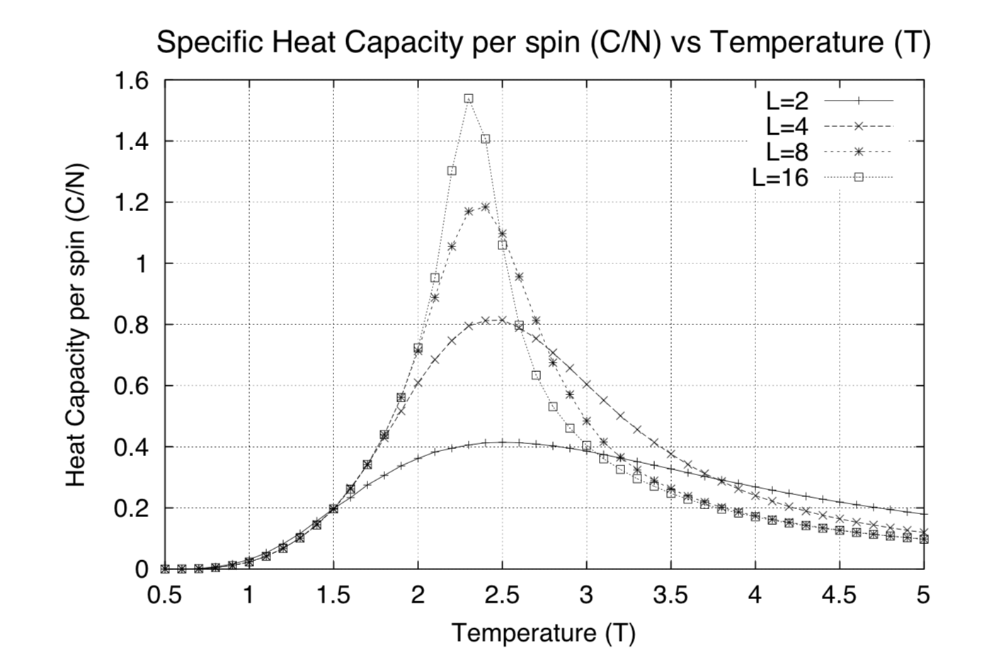
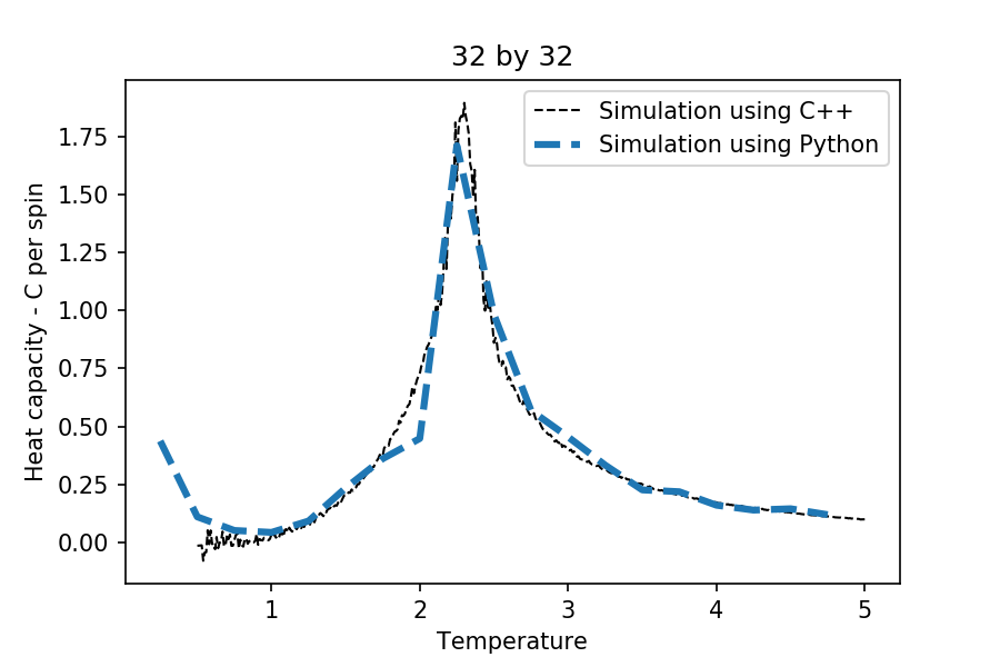
This was found to fit very well with the C++ data given and literature (see above^[1]), including the Curie temperatures and the shape of the plots at different lattice sizes. The phase transition is characterised as a second order phase transition based on the discontinuity of the second order derivative properties of the system. One of which is the heat capacity at constant volume. Hence, from the plot above, the temperature at which phase transition occurs (Curie temperature) can be identified easily compared to trying to identify such temperature from the energy/magnetization per spin against temperature plots. Although, because of the limitation of the Ising Model, you don't get a clear divergence at the phase transition (of the heat capacity plots) as we're supposed to for a second order phase transition. Hence, for now, the peak of the heat capacity for each of the plots must be a possible divergence point.

As you can see from the plot above, the heat capacity at the temperature well below the Curie temperature seems to have significant rise in its value (suppose to be zero). One explanation to this involves the problem with the Ising model itself, due to the fact that the lattices used are of a finite size. Spontaneous spin flipping was found to be prominent in the systems at temperature well below the Curie temperature. This cause fluctuations in the magnetization and the energy of the system, increasing the variance of the energies at the lower temperatures. Since the heat capacities were calculated from the variance of the energy, this explains why the heat capacities shoot up at the very low temperatures. This obviously contradicts with what was expected, as the magnetisation and energy were suppose to be stable.^[2]Another possible explanation is that the system at low temperature reaches a 'metastable' state (as mentioned in the previous section). After spending time to explore this phenomenon, it was found that eventually it will reach the equilibrium. Although, this took much more cycles to reach equilibrium compared to the normal cases, affecting the mean average and variance calculations, affecting the heat capacities at low temperatures.

Task 17

TASK: A C++ program has been used to run some much longer simulations than would be possible on the college computers in Python. You can view its source code here if you are interested. Each file contains six columns:
$T, E, E^{2}, M, M^{2}, C$
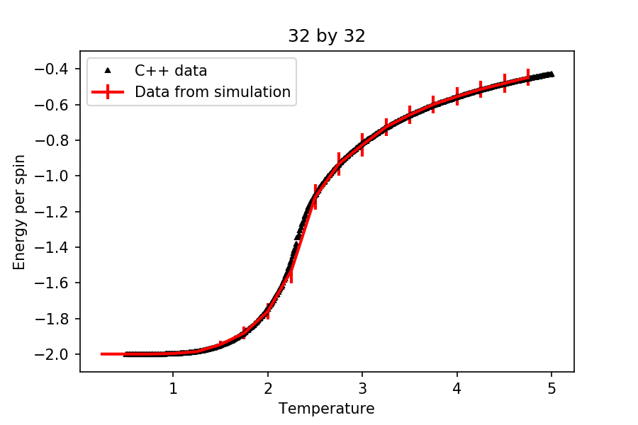
(the final five quantities are per spin), and you can read them with the NumPy loadtxt function as before. For each lattice size, plot the C++ data against your data. For one lattice size, save a PNG of this comparison and add it to your report — add a legend to the graph to label which is which. To do this, you will need to pass the label="..." keyword to the plot function, then call the legend() function of the axis object (documentation here).

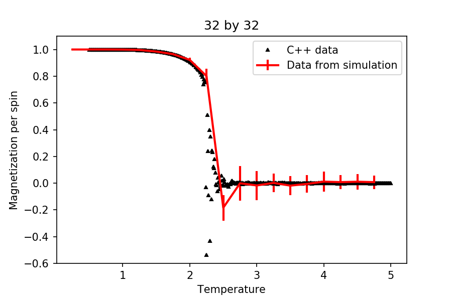
All the data from the simulation was found to match the C++ data given very nicely. Further investigations also revealed that running the simulation through more temperatures result in very noisy data. This subsequently affected the calculation of the heat capacity, resulting in mismatch of the simulation data and the C++ data given. Unless more steps were used in running the simulation, increasing the number of temperatures would not help improve the results obtained.

Task 18

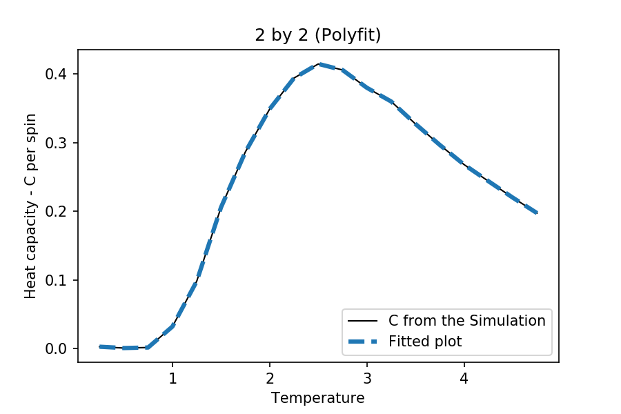
TASK: write a script to read the data from a particular file, and plot C vs T, as well as a fitted polynomial. Try changing the degree of the polynomial to improve the fit — in general, it might be difficult to get a good fit! Attach a PNG of an example fit to your report.

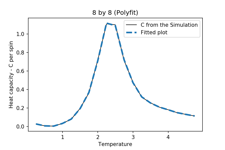
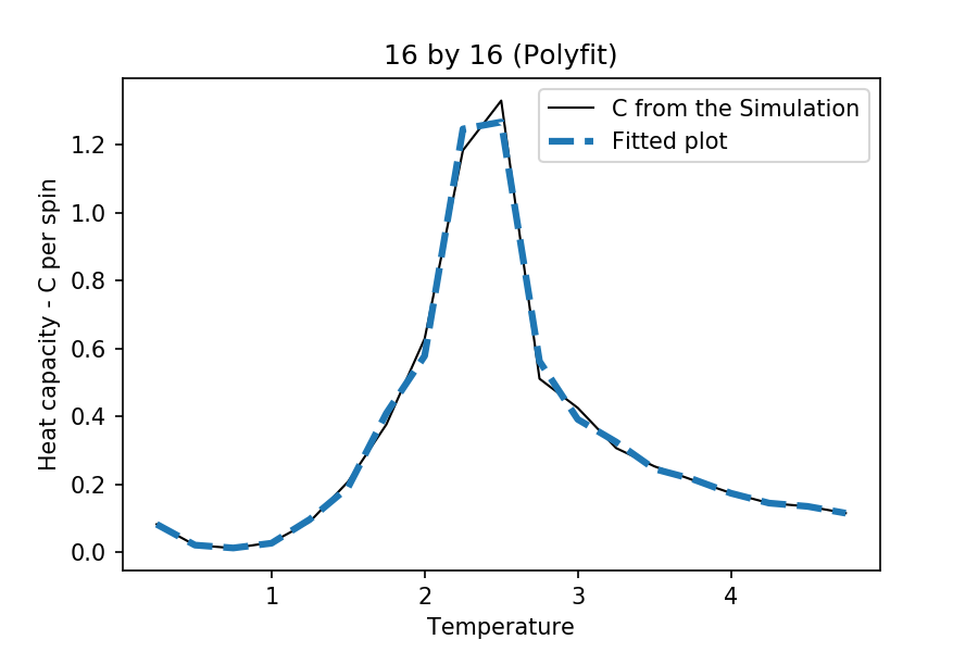
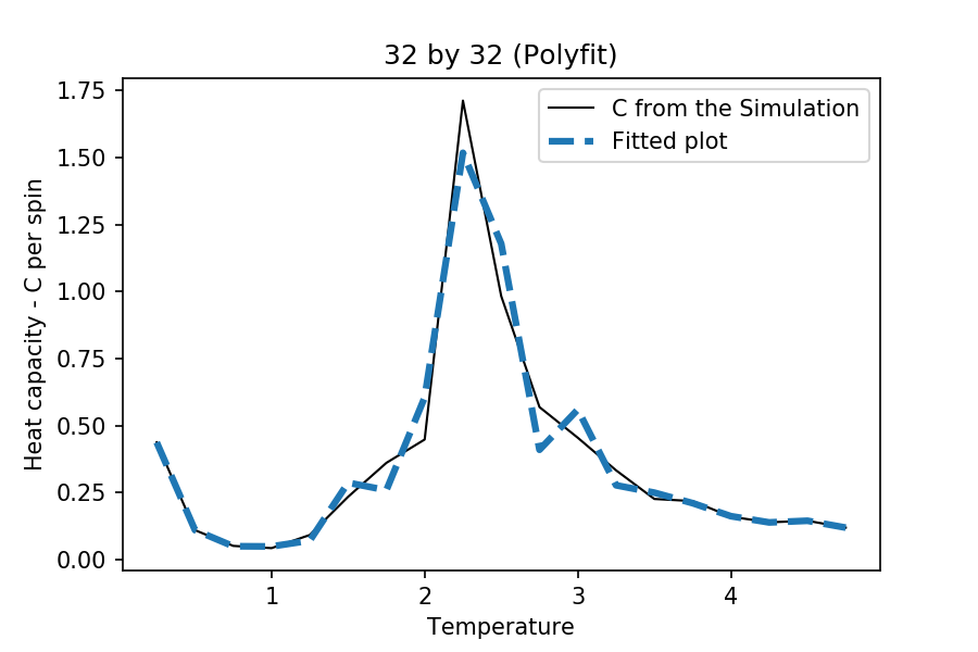
The degree of polynomial used here is at 20. It was later realized that this was not neccessary, as the point of the fitting was to obtain a plot that represents how the original graph was suppose to look like. Although, a good fitting is hard to achieve when all the data points were included. The next section only fits certain range in the plots at the critical region.

Task 19

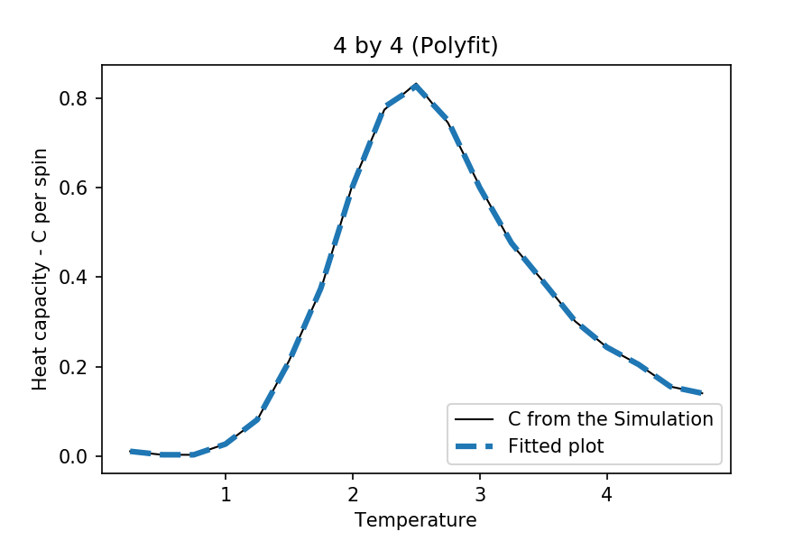
TASK: Modify your script from the previous section. You should still plot the whole temperature range, but fit the polynomial only to the peak of the heat capacity! You should find it easier to get a good fit when restricted to this region.

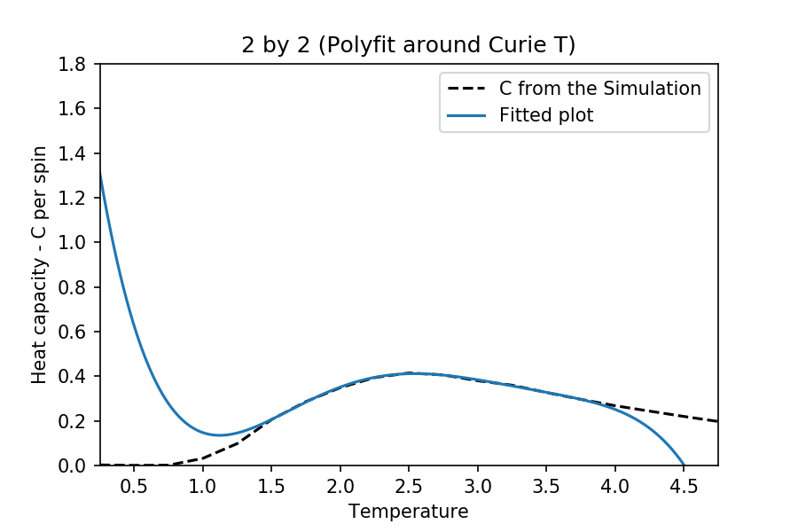
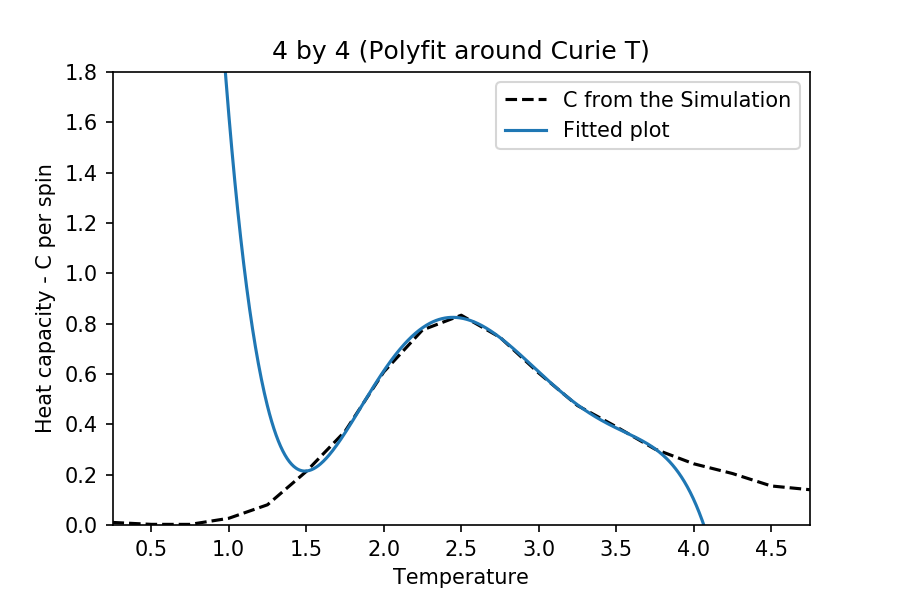
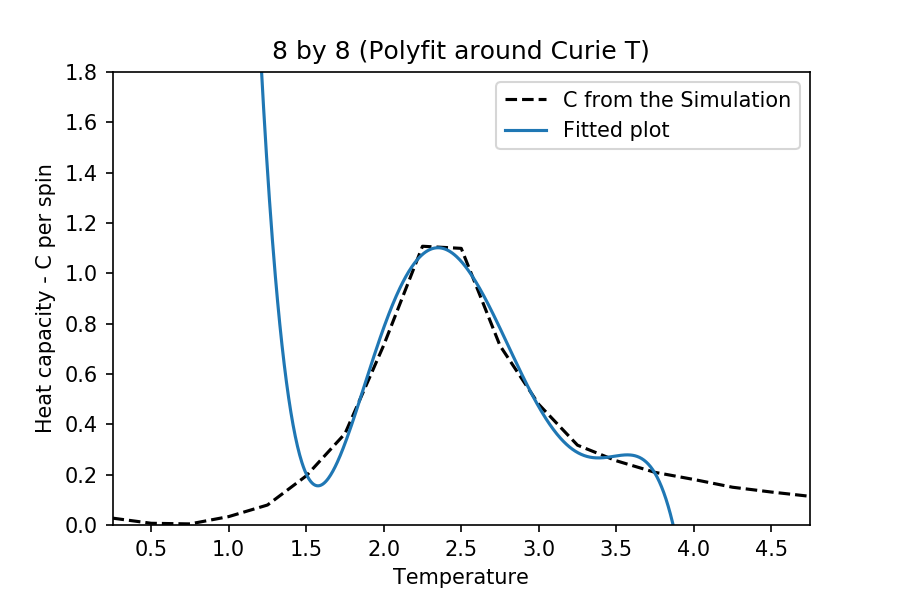
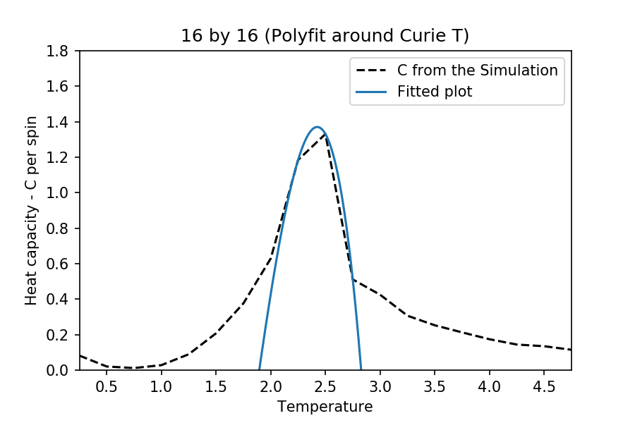
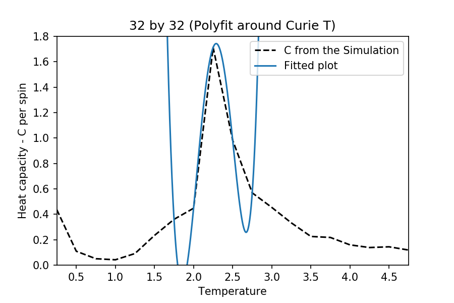
The interval of the $T_{m i n}$ and $T_{m a x}$ are different for each case. This is to make sure that there are enough points for the function to work, but at the same time obtain a better fitting near the critical temperature. The degree of polynomial used for each case is 5. The following are the temperature range used for the each different cases:

$2 \times 2$ : $2.00 < T < 3.00$

$4 \times 4$ : $2.00 < T < 3.00$

$8 \times 8$ : $2.00 < T < 3.00$

$16 \times 16$ : $2.00 < T < 2.75$

$32 \times 32$ : $2.00 < T < 2.50$

Also, note that the graph fitting here does not exactly match the original plots obtained (as it is not supposed to). Although, it fits such that the best possible Curie temperature and the peaked heat capacities are obtained (compared to literature).

The maximum values for the heat capacities at different lattice sizes are as follows:

$2 \times 2 = 0.41$ at $T = 2.55$

$4 \times 4 = 0.83$ at $T = 2.45$

$8 \times 8 = 1.10$ at $T = 2.35$

$16 \times 16 = 1.37$ at $T = 2.40$

$32 \times 32 = 1.74$ at $T = 2.29$

Task 20

TASK: find the temperature at which the maximum in C occurs for each datafile that you were given. Make a text file containing two colums: the lattice side length (2,4,8, etc.), and the temperature at which C is a maximum. This is your estimate of
$T_{C}$
for that side length. Make a plot that uses the scaling relation given above to determine
$T_{C, \infty}$
. By doing a little research online, you should be able to find the theoretical exact Curie temperature for the infinite 2D Ising lattice. How does your value compare to this? Are you surprised by how good/bad the agreement is? Attach a PNG of this final graph to your report, and discuss briefly what you think the major sources of error are in your estimate.

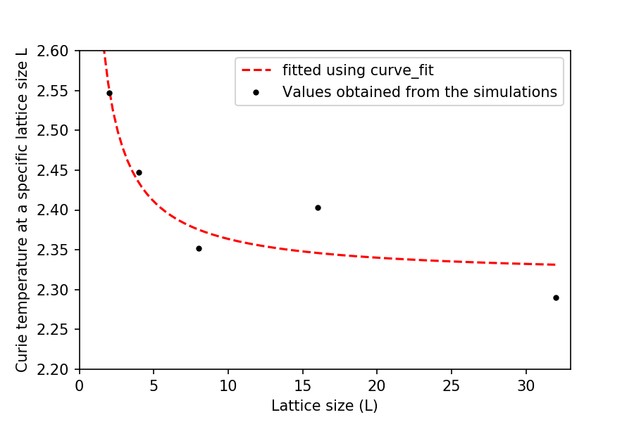
This fitting model was used to determine the Curie temperature for lattice where the L size is at infinity. This is because of the problem of the Ising model mentioned earlier, even after the problem was minimized by using periodic boundary conditions. np.curve_fit was used to fit the data from the simulation, using the equation given in the script $T_{C, L} = \frac{A}{L} + T_{C, \infty}$ .

By fitting the Curie temperatures obtained from the simulations, the Curie temperature for an infinite lattice was found to be $T_{c} = 2.317 \pm 0.013$ . This is very similar to the value calculated analytically using the Kramers–Wannier duality method (2.106 % difference), with the value of $T_{C} = 2.2692$ .^[3]This is definitely a viable and an efficient alternative to exact calculation and the experimental error is very small.

This is surprising as the temperature range used for each lattice sizes could have been much more to increase the reliability of the results. If more time were given, together with faster and better computing power, data with higher quality and more repeats could have been obtained. There are many errors regarding the simulations carried out. One of which is the fact that sometimes, it was observed that the lattice system reached a 'metastable' state. This is not the lowest energy state and this will have definitely affected the subsequent calculations and analysis. In addition to this, it was found that it can take quite a few cycles for the simulation to run before reaching equilibrium. Especially for the $32 \times 32$ system at $T = 0.25$ , where it takes around 100,000 cycles to reach equilibrium. Sometimes it takes more than this. Based on literature found, it was common to run for a total of 1,000,000 cycles to obtain a value from a single temperature (for lattice sizes less than 16 by 16). Another error in the Ising model (as described before) is the fact that spontaneous spin flipping is possible at temperatures below the Curie temperature, causing problems in the analysis of the results obtained. More simulations can also be carried on bigger lattice sizes, so that more $T_{C, L}$ can be used in the np.curve_fit, which would yield a better fitting and could make the values obtained closer to the values obtained analytically.

Possible extensions

There are many possible extensions in which you can carry out to further understand the properties of materials. This include:

Determine the magnetic susceptibility of the data already obtained from the simulations.

Introducing coupling constant to the simulations and try out different values for this.

Expand this to three dimensional systems and deduce its phase transition temperatures and other critical properties.

Try simulating alloys using the Ising Model and compare with results from analytical methods.

Source code

import numpy as np
class IsingLattice:
   E = 0.0
   E2 = 0.0
   M = 0.0
   M2 = 0.0
   n_cycles = 1
   def __init__(self, n_rows, n_cols):
       self.n_rows = n_rows
       self.n_cols = n_cols
       self.lattice = np.random.choice([-1,1], size=(n_rows, n_cols))

   def energy(self):
       "Return the total energy of the current lattice configuration."
       #I used the np.multiply, np.roll and np.sum to calculate the energy in one go
       return (-1)*(np.sum((np.multiply(self.lattice, np.roll(self.lattice,1,axis=0))
                    +np.multiply(self.lattice,np.roll(self.lattice,1,axis=1)))))

   def magnetisation(self):
       "Return the total magnetisation of the current lattice configuration."
       #This is simply by using the np.sum functions to add up all the spins in the lattice
       return np.sum(self.lattice)

   def montecarlostep(self, T):   
       energy = self.energy()
       random_i = np.random.choice(range(0, self.n_rows))
       random_j = np.random.choice(range(0, self.n_cols))  
       random_number = np.random.random()          
       #code starts here - flip a random lattice point
       if self.lattice[random_i,random_j] == 1:
           self.lattice[random_i,random_j] = -1
       else:
           self.lattice[random_i,random_j] = 1
       #here I compare their energy
       dE = self.energy() - energy   
       #Here I decide whether to flip back the spin or leave it using the algorithm given in the script
       if dE <= 0:
           energy = self.energy()
       elif random_number <= np.exp((-dE)/(T)):
           energy = self.energy()  
       else:
           if self.lattice[random_i,random_j] == 1:
               self.lattice[random_i,random_j] = -1
           else:
               self.lattice[random_i,random_j] = 1
       #here I decide how many initial cycles to discard - note that this is different for different lattice sizes to save time
       if self.n_cycles <= 250000:
           self.E = self.E
           self.E2 = self.E2
           self.M = self.M
           self.M2 = self.M2
       else:
           self.E+= self.energy()
           self.E2 += self.energy()**2
           self.M += self.magnetisation()
           self.M2 += self.magnetisation()**2
       self.n_cycles +=1
       energy = self.energy()
       magnetisation = self.magnetisation() 
       return energy,magnetisation

   def statistics(self):
       self.E_ = self.E/(self.n_cycles-250000)
       self.E2_ = self.E2/(self.n_cycles-250000)
       self.M_= self.M/(self.n_cycles-250000)
       self.M2_ = self.M2/(self.n_cycles-250000)  
       return self.E_,self.E2_, self.M_, self.M2_, self.n_cycles

References

↑ Kotze, Jacques. "Introduction to Monte Carlo methods for an Ising Model of a Ferromagnet." arXiv preprint arXiv:0803.0217 (2008). APA
↑ Kotze, Jacques. "Introduction to Monte Carlo methods for an Ising Model of a Ferromagnet." arXiv preprint arXiv:0803.0217 (2008). APA
↑ H. A. Kramers and G. H. Wannier, Physical Review, 1941, 60, 252–262.

[1] Kotze, Jacques. "Introduction to Monte Carlo methods for an Ising Model of a Ferromagnet." arXiv preprint arXiv:0803.0217 (2008). APA

[2] Kotze, Jacques. "Introduction to Monte Carlo methods for an Ising Model of a Ferromagnet." arXiv preprint arXiv:0803.0217 (2008). APA

[3] H. A. Kramers and G. H. Wannier, Physical Review, 1941, 60, 252–262.

[1]

[2]

[3]