Rep:Mod:ZC2814liqsim
Abstract
This experiment used computational method to simulate a simple liquid model using Lennard-Jones potential and velocity-Verlet algorithm. A number of observables were output and compared to realistic liquids to justify the accuracy of the model system generated by this method.
Introduction
Velocity-Verlet algorithm
Velocity-Verlet is one modified edition of Verlet's algorithm with approximations and good precision. We wanted to simulate a real liquid system from knowing the starting positions of atoms and their velocities at the same time, so velocity-varlet algorithm was used. Firstly we set up a collection of N atoms which behave as classical particles and each one of them interacted with every atom else in the system. So every atom felt a force. As in Newton's second law F=am and its differential equations, if we know how the force, F, changes with respect to time, we can know the position and velocity of an atom in the system at any time by solving the equation relating to that atom.
- is the force acting on atom i.
- is the mass of atom i.
- is the acceleration of atom i at time t.
- is the velocity of atom i at time t.
- is the position of atom i at time t.
Instead of solving with positions, velocities and forces as continuous functions with respect to time, they can be break up into changes with a sequence of timesteps with length . By adding up the Taylor expansions of the positions for a single atom at its next tilmestep and one timestep backwards followed by substitution of Newton's second law, we arrive at:
The Newton's law for these atoms can be solved by Verlet's algorithm, however, this methods does not output velocities therefore we cannot calculate kinetic energies. Velocity-Varlet algorithm comes up to get around this problem. We assume that the acceleration of an atom only depends on its position. W can now calculate atomic velocities explicitly. Velocity-Verlet algorithm has its form with an accuracy up to :
Atomic Forces
As we were simulating a simple liquid with only one type of atom, Lennard-Jones potential would be able to model the interactions between atom pairs.
It can also be expressed in standard 12/6 form:
In this equation, is the potential well depth, is the distance where the potential between the pair of particles is zero and r is the distance between the pair of particles.
Force is the negative derivative of potential energy. When the equation of force in terms of the Lennard-Jones potential is zero,, the equilibrium is reached and the resultant force is also zero:
The LJpotential at is:
, therefore:
Periodic Boundary Conditions and Truncation
We enclose the atoms created in a cubic simulation "box" with fixed dimensions, and set the lattice type of the melting crystal and density of lattice unit. This can be related to realistic systems when applying this to e.g. water system:
Density of water= under standard consitions (298K, 1atm). So the total mass of 1 mL water= 1g. The number of moles of water molecules=
Total number of molecules in 1 mL of water=
The volume of 10,000 molecules of water=
The initial position of atom is . After it moves along the vector , the position should be . Applying the periodic boundary of to , the position should be .
Reduced Units
Reduced units were used throughout the experiment as Lennard-Jones interactions were used.
- distance
- energy
- temperature
For example, the Lennard-Jones parameters for argon are.When LJ cutoff is, in real units it will be:
The well depth in kJ/mol will be:
And the reduced temperature in real units will be:
Aims and Objectives
We aimed to simulate a single-specied liquid system by melting a crystal which closely represents a real liquid system. As we were starting from assigning every atom its initial position and initial velocity, velocity-Verlet algorithm was used for simulation. Pressure changes and density changes as a function of temperature was output and compared with real systems at NpT and NVT ensembles respectively. The simulation would then be extended to vapour and solid, to see if any differences between realistic gas, liquid and solid phases could be observed.
Methods
TIME STEP
Melt_crystal.in was used as template and run at timesteps 0.001, 0.0025, 0.0075, 0.01 and 0.015 repectively by LAMMPS on HPC. Output log files were saved as .txt and trajectory files saved as .lammptrj.
NpT ensemble
Simple cubic lattice crystal generated with density 0.8. Cubic simulation box “box” extending 10 lattice spacings from origin in x, y and z directions containing only one type(type 1) of atoms was generated. Mass of type 1 atoms was set at 1.0. Interaction set at pairwise standard 12/6 Lennard-Jones potential without Coulombic interaction, with a cutoff distance 3.0 with lines:
pair_style lj/cut 3.0
Pairwise force field between any pair of atoms was set at 1.0.
pair_coeff * * 1.0 1.0
Initial velocities were assigned to every atom created at temperature “variable T” fulfilling Maxwell-Boltzmann distribution. How much time simulated so far, total energy of the atoms, temperature and pressure were output by LAMMPS every 10th timestep. Timestep was set at 0.001, total timestep equaled 100000 which meant 100 time units was simulated.
### SPECIFY TIMESTEP ###
variable timestep equal 0.001
variable n_steps equal floor(100/${timestep})
timestep ${timestep}

### RUN SIMULATION ###
run ${n_steps}
run 100000
Timestep set up was written as above, instead of:
timestep 0.001
run 100000
This was to define a variable "timestep" so the numerical timestep did not need to be changed manually when it needed to be changed and more than one tilmestep can be run in sequence in a single script if wanted. Temperature chosen to run were 2.0, 2.2, 2.4, 2.6, 2.8 simulated at pressure 2.6 or 5.0 respectively. Values of density, pressure and temperature would be sampled every 100 timesteps for an average value. 1000 values were sampled for every variables listed above over 100000 timesteps. These ten .in files were run by LAMMPS on HPC and output log files were saved.
NVT ensembles
npt.in was taken to be modified into NVT ensemble(modified nvt.in is attached as appendix). Equilibrium was generated by melting a crystal and all npt in script changed by nvt. Thermostat was turned off once the system was in correct thermodynamic state. 0.001 timestep was used to run 100000 timesteps. Average temperature calculated from values of every 100 timesteps and heat capacity was output by LAMMPS at input temperature 2.0, 2.2, 2.4, 2.6 and 2.8 for density 0.2 or 0.8 respectively, 10 simulations in total.
RDF
liq.in at density=0.8, temperature=1.2 was used as a template for running vap.in and sol.in. for vapour and solid systems. vap.in had density=0.4, temperature=1.2 while sol.in had density=1.6, temperature=1.2 and lattice type fcc instead of sc. 3 systems were run by LAMMPS on HPC. g(r) and intergration of g(r) with respect to r were calculated by VMD using output trajectory files.
MSD
liq(2).in with density=0.8 and temperature=1.2 was used as template for running vap(2).in and sol(2).in. The two input files were modified by same steps as RDF. 3 systems were run by LAMMPS on HPC. MSD files and VACF files were saved.
Results and Discussion
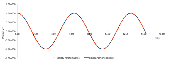
Single-specied system was generated as it would be simpler to only consider interaction between same kind of atoms. Velocity-Verlet algorithm was used to approximately solve LJ potential mode at tilmestep 0.1, 0.2 and 0.3. The results were compared with calculations from classic harmonic oscillator. Errors accumulated with increasing time so simulations of long periods was discouraged. Examining equilibrium with small time steps and short real time showed that equilibrium could be achieved very shortly after the simulation started. Therefore short time period would be encouraged. From these results, only timestep smaller than 0.2 could achieve total energy changes less than 1%.


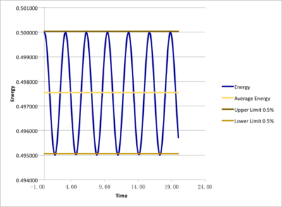
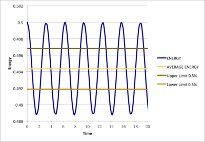
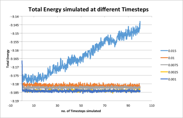
Smaller different timesteps(0.001, 0.0025, 0.0075, 0.01, 0.015) were examined as to determine a suitable timestep for further simulations and outcame total energies were under comparison. Monitoring total energy numerically was important as we needed to make sure our simulated system fulfilled energy conservation, correctly modelling real systems. From the results, 0.0025 and 0.001 would be suitable. However, even the 0.001 timestep task here took less than 10 minutes to simulate, so 0.001 was chosen for further simulations for more detailed and accurate results.
Simulation boxes were created with commands to enclosure the atoms. The system was not started from assigning random positions to every atom, but started from melting a crystal structure as two atoms may be generated too close to each other or might even collide. We were running the simulation under Lennard-Jones interaction, so repulsive force and potential energy would shoot up and unstabilize the system. Further more, crystal structures were highly ordered and it would be quite easy to assign positions to atoms once one atom was assigned. This was made even easier by creating simple cubic lattice with dimension 10 in x, y and z from origin instead of other ones. The side length of the simulated box was 1.07722 in the output file. If a face-centred cubic lattice with a lattice point number density of 1.2 was simulated, the side length of the cubic unit cell would be and 4000 atoms would be created.
System kept number of atoms, pressure and temperature constant were simulated in the NpT ensemble session. During the simulation, temperature was controlled to satisfy target temperature by adjusting so that the temperature was correct if every velocity was multiplied by this constant.
In the system with N atoms, each with 3 degrees of freedom:
By multiplying every velocity by and substituting T with we can get the second equation:
By substituting (2) we can get:
Densities were calculated by and this was plotted as a function of temperature. Densities corresponded to certain temperature and pressure were also calculated form Ideal Gas Law from method below for comparison:
Starting from Ideal Gas Law equation and reduced unit equations from Introduction,
As , and [1], so by substitution:
The results showed that the simulated densities were much lower than the IGL densities however same decreasing trend was observed against temperature. This is because the Ideal Gas Law assumes that there is no interaction between molecules and the repulsive force between the molecules is zero. Molecules in Ideal Gas system can be compressed to a great extent, making the volume occupied very small for a given volume. Therefore the density can be higher. In the Lennard-Jones model, the molecules will interact with each other when they come too close to each other and the repulsive force arises with decreasing distance. Therefore for a given volume the molecules will rather stay far apart and the density would be lower .
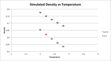

The discrepancy also increases with pressure. At lower pressures, the intermolecular distance is large and densities do not change as much percentage as at high pressures.
System kept number of atoms, volume and temperature constant were simulated in the NVT ensemble session. Heat capacity calculation was put into the input script:
is the variance in , is the number of atoms, and it is a standard result from statistics that .
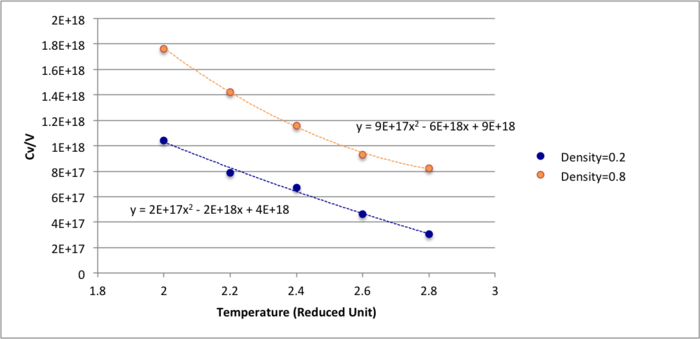
Heat capacity can be understood as how far the system is able to fluctuate from its average equilibrium temperature, as well as total energy. As the results shown above, smaller time step would lead to smaller fluctuation therefor stable system and very large heat capacity. This is because the lattice energy gap decreases with increasing temperature, so less energy will be required. This indicates that heat capacity is proportional to energy as shown in the equation. Also, it is shown that the lower the density, the lower the heat capacity. The reason could be high density meant the particles would be closer together in a lower volume and energy transfer between atoms would be faster, therefore less heat is required to heat the system. For the same number of particles with lower density, atoms would be further apart and would need more energy to heat up.

The radial distribution function was plotted for vapour, liquid and solid phases. The densities and temperatures were chosen from Lennard-Jones phase diagram to fulfil the system states. The radial distribution function indicates the probability of finding a nearest neighbor from a particle and would reveal the phase of the system simulated. The RDFs for the three systems are very different. The solid has the largest number of peaks followed by liquid and then gas. The peaks represent the density around each atom and hence solid which has the highest density will have more peaks. The peaks in the solid phase has decreasing amplitude with increasing r. It can be seen that the probability of finding a particle between the first and second peak is zero. This is because particles in solid phase do not have brownian motion and can only vibrate in fixed positions. The solid phase has long and short range order and this can be indicated by the peaks. The short range order is shown by the first three tall peaks and the long range order is shown by the smaller peaks behind.The RDF of the liquid phase has three peaks with decreasing amplitude as r increases. The wider peaks mean that the liquid phase is more disordered than the solid phase.The decreasing amplitude with increasing interatomic separation indicates that the Brownian motion of particles in the liquid phase makes the order decrease with increasing separation. The three peaks indicate that the liquid phase only has short range order. The RDF of the gas phase only has one broad peak. This suggests the gas phase is highly disordered and there is no short nor long range order.In the RDF of the solid phase, the first three peaks correspond to the nearest neighbor of the referenced particle, the second nearest particle and the third nearest particle respectively. The lattice spacing is the distance between the zero probability minima and is 1.275 in reduced units.
 |
 |
 |
 |
 |
 |
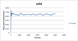
The liquid simulation corresponded to a real liquid as MSD increased linearly with simulation time as the atoms moved in Brownian motion. The vapour simulation was also linear for the most part as it also resembles a brownian motion. The first curve bit raised from the random collision of vapour atoms as they were very far apart and the probability, or frequency, of collisions would be quite small. Thus needed some time to establish this statical equilibrium. For solid phase, atoms only move around a fixed position and the MSD reached constant average value at around 200 tilmestep. The simulation illustrated these information satisfyingly. By comparing 3375 atom system to 1 million atom system, clearly the 1 million system gave better stable results as there were more atoms and more collisions could be sampled and data would meet statistical requirement better.
Conclusion
Liquid system was simulated with enclosure simulation box under Lennard-Jones potential by velocity-Verlet algorithm. Suitable timestep 0.001 was evaluated while total energy, pressure and density changes with temperature were monitored. The outcome was quite satisfying with same trend and small value differences compared to other approximation methods e.g. Ideal Gas Law. The simulation method was then used to model vapour and solid. Radial distribution function g(r) and MSD was examined. Both parameters showed good representation of real systems and gave differences between liquid, vapour and solid phases. Therefore the simulation preformed in this experiment was satisfying.
Appendix & References
variable density equal 0.2

### DEFINE SIMULATION BOX GEOMETRY ###
lattice sc ${density}
region box block 0 15 0 15 0 15
create_box 1 box
create_atoms 1 box

### DEFINE PHYSICAL PROPERTIES OF ATOMS ###
mass 1 1.0
pair_style lj/cut/opt 3.0
pair_coeff 1 1 1.0 1.0
neighbor 2.0 bin

### SPECIFY THE REQUIRED THERMODYNAMIC STATE ###
variable T equal 2.0
variable v equal 16875
variable timestep equal 0.001

### ASSIGN ATOMIC VELOCITIES ###
velocity all create ${T} 12345 dist gaussian rot yes mom yes

### SPECIFY ENSEMBLE ###
timestep ${timestep}
fix nve all nve

### THERMODYNAMIC OUTPUT CONTROL ###
thermo_style custom time etotal temp press vol
thermo 10

### RECORD TRAJECTORY ###
dump traj all custom 1000 output-1 id x y z

### SPECIFY TIMESTEP ###

### RUN SIMULATION TO MELT CRYSTAL ###
run 10000
unfix nve
reset_timestep 0

### BRING SYSTEM TO REQUIRED STATE ###
variable tdamp equal ${timestep}*100
variable pdamp equal ${timestep}*1000
fix nvt all nvt temp ${T} ${T} ${tdamp}
run 10000
reset_timestep 0

### MEASURE SYSTEM STATE ###
thermo_style custom step etotal temp press atoms density vol
variable dens equal density
variable dens2 equal density*density
variable temp equal temp
variable temp2 equal temp*temp
variable press equal press
variable press2 equal press*press
variable N equal atoms
variable N2 equal atoms*atoms
variable E equal etotal
variable E2 equal etotal*etotal
fix aves all ave/time 100 1000 100000 v_dens v_temp v_press v_dens2 v_temp2 v_press2 v_E v_E2
unfix nvt
fix nve all nve
run 100000

variable avedens equal f_aves[1]
variable avetemp equal f_aves[2]
variable avepress equal f_aves[3]
variable errdens equal sqrt(f_aves[4]-f_aves[1]*f_aves[1])
variable errtemp equal sqrt(f_aves[5]-f_aves[2]*f_aves[2])
variable errpress equal sqrt(f_aves[6]-f_aves[3]*f_aves[3])
variable heatcapacity equal ${N2}*(f_aves[8]-f_aves[7]*f_aves[7])/(1.38064852e-23*f_aves[5])

print "Averages"
print "--------"
print "Temperature: ${avetemp}"
print "Stderr: ${errtemp}"
print "Pressure: ${avepress}"
print "Stderr: ${errpress}"
print "heatcapacity: ${heatcapacity}"
- ↑ http://www4.ncsu.edu/~franzen/public_html/CH795N/modules/ar_mod/comp_output.html
