Jack Dawson - Yr3 Comp: Liquid Sim.

Not a bad attempt, although slightly uncomplete. You've attempted to give physical explanations for observed phenomena and generally I think you've understood the material to a good standard. Mark: 63/100

1 Theory

1.1 Task

Compltete the Classical Harmonic Osciallator Spreadsheet

File:JmsD HO.xls

1.2 Task

For δt=0.01, estimate the positions of maximum error and fit accordingly.

Figure 1.1 shows how the maximum error increases linearly. This can be rationalised by the fact that each cycle of simulation follows on from the last, so the error of the new cycle is combined to the uncertainty in a previous calculation for an older timestep and so on. Tick

1.3 Task

Experiment to find the timestep range to ensure the total energy does not change by more than 1% over the course of the simulation. Why is this important?

In simulations such as this, the physical model is considered an isolated system. We are modeling the changes in velocity and thus kinetic energy changes of induvidual particles/atoms over a total timeframe at constant timesteps. As such, the particles are moving around, interacting, transfering energy between each other. However, unless we are changing variables such as Temperature, Number of particles, Volume (density) etc. during a simulation, the overall energy should remain constant. Therefore it is important to monitor the total energy to ensure our model is fitting with our physical understanding.

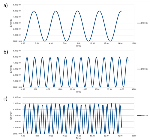
From experimentation, it can be seen that to limit this total energy change over a simulation, the time step should really be smaller than 0.3. It can be seen in Figure 1.2 how the peaks and thus total energy begin to fluctuate significantly more for 0.3 and above.It's more like 0.2 but right idea

1.4 Task

Maths based upon a single Lennard-Jones interaction

Tick

1.5 Task

Estimate the number of water molecules in 1 mL under standard conditions.

Density of water = 1 g/ml Molecular weight of wate = 18 g/mol Moles in 1 ml, n = 1/18 Number of molecules = n x N_A = 1/18 x 6.022x10²³ 3.35x10²²

Tick

Estimate the volume of 10000 water molecules under standard conditions.

10000/N_A = moles of water, n Mass of 10000 water molecules, m = n x 18 The volume, V = m / 1 g/ml 2.99x10^-19

Tick

1.6 Task

Consider an atom at position (0.5, 0.5, 0.5) in a cubic simulation box which runs from (0, 0, 0) to (1, 1, 1). In a single timestep, it moves along the vector (0.7, 0.6, 0.2). At what point does it end up, after the periodic boundary conditions have been applied?.

The particle should end up in position (0.2,0.1,0.7) after the application of periodic boundary conditions.

This is because, if the number of particles in the box remains constant, if a particle excit the box on one face, it will return from the opposite. In this case, if the particle starts at (0.5,0.5,0.5) in the cubic box ((0,0,0):(1,1,1)) and moves along the vector (0.7,0.6,0.2), it will reappear from the other face, positioned now at (0.2,0.1,0.7).Tick

1.7 Task

The LJ parameters for argon are $σ$ = 0.34 nm, $ϵ / k_{B}$ = 120 K. If the LJ cutoff is r* = 3.2, what is it in real units? What is the well depth in kJ mol^-1? What is the reduced temperature T*=1.5 in real units?

r = 1.088 x10^-10 m

Should be E-9 but again right idea

T = 180 K

Tick

ϵ

= 0.014 kJmol^-1

not quite right, 0.997 kJ mol^-1

2 Equilibriation

2.1 Task

Why do random starting coords cause problems in simulations If particles are placed randomly, there is chance for multiple particles to be placed in the same positions, or at least close too each other. It two particles are close or overlap, there would be very strong resulting interactions. These large forces would caus the model to deviate from its classical behaviour, and will affect properties from energy, to timestep. It doesn't deviate from classical behviour just the energies are so large that the corresponding timestep should be unreasonably small for a simulation without "blow-up"

Therefore it is wise to start a liquid or gas simulation as a 'melt' from particles on lattice points (which can allow random positioning to some degree), e.g. Simple cubic. This ensures particles will begin a suitable distance away from each other.

2.2 Task

Prove that lattice spacing of 1.07722 gives a number density of 0.8

If lattice spacing is 1.07722, Volume of one cube = 1.07722³ If number density is Number / Volume, and there is one particle per cube, number density = 1 / Volume 1 / 1.07722³ = 0.79999

Tick

If instead FCC, and number density of 1.2, what is the length of the cubic uni cell?

First calculate Volume of the cell: V = Number / number density The Number of particles in a FCC unit cell are 4, so V = 4 / 1.2 The cube root of the volume will give side length... (4/1.2)^1/3 = 1.4938

Tick

2.3 Task

For the FCC latice, how many atoms would be created by create_atoms

Assuming no other parameters (i.e. the box size [Below]) have changed...

region box block 0 10 0 10 0 10
create_box 1 box

There should be 4000 atoms created.

If there are 1000 atoms in a 10x10x10 box for a sc lattice that has one atom per unit cell, a lattice such as FCC that has 4 atoms per unit cell should yield 4000 atoms. Tick

2.4 Task

Find and explain the purpose of:

mass 1 1.0
pair_style lj/cut 3.0
pair_coeff * * 1.0 1.0

mass - Sets the mass for the types of atoms, argument(1) is the type, argument(2) is the mass.
pair_style - Calculates the pair interactions (pair potentials defined as interactions between atoms within a certain distance), argument(1) "lj/cut" means this line refers to the global cutoff for all Lennard-Jones interactions, argument(2) defines the distance.
pair_coeff - Provides the interaction coefficients for the interactions between atoms, arguments(1 & 2) refer to the attoms that interact (* means all types 1->N), and arguments (3 & 4) are those coefficients.Tick

2.5 Task

Given that we are specifying x_i and v_i, which integration algorithm is to be used?

The Velocity-Verlet Algorithm

2.6 Task

### SPECIFY TIMESTEP ###
variable timestep equal 0.001
variable n_steps equal floor(100/${timestep})
variable n_steps equal floor(100/0.001)
timestep ${timestep}
timestep 0.001

### RUN SIMULATION ###
run ${n_steps}
run 100000

The second line (starting "variable timestep...") tells LAMMPS that if it encounters the text ${timestep} on a subsequent line, it should replace it by the value given. In this case, the value ${timestep} is always replaced by 0.001. In light of this, what do you think the purpose of these lines is? Why not just write:

timestep 0.001
run 100000

The purpose of using ${timestep}, or for any other variable for that matter, is that it allows for that property in the simulation to be changed just once in the input file, as opposed to the file being manually altered on every line that variable is called.Tick

2.6 Task

Plot Energy, Temperature and Pressure vs Time for timestep = 0.001

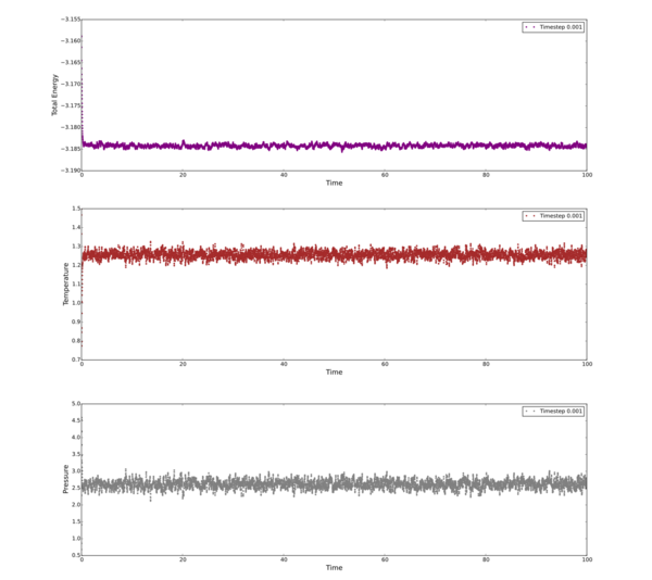
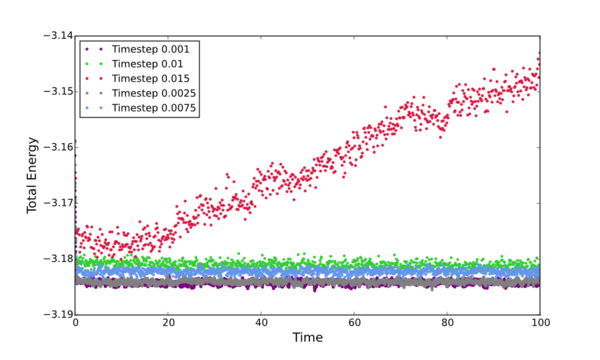
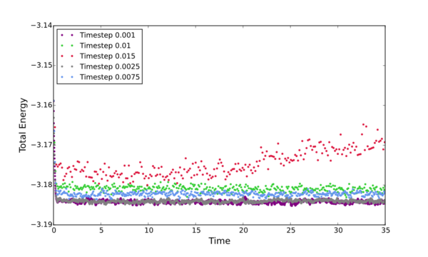
Plot all the inital simulations as Energy vs Time, discus the best timestep to progress with.

The timestep chosen for ongoing calculations was 0.0025. The reason being that it was one of only two that provided data showing convergence within the full simulation time (Energy vs Time graph). Of these two timesteps - 0.0025 and 0.001 - the 0.0025 is the better choice to progres with due to it's slight advantage in computational efficiency. The larger the time step, the fewer data points collected.

[A note should be made about te 0.15 timestep - This is quite clearly a bad choice because instead of converging it diverged...] Tick but why do we see this trend of tot eners vs timesteps?

3 Simmulations under specific conditions

3.1 Task

Choose 5 temperatures (above the critical temperature, T* = 1.5), and two reasonable pressures in Lennard-Jones units.

Run these simulations to plot the 'Equations of State' [Below].

The 10 phase points used inn this task were determined by the 5 temperatures (T): 1.6, 1.8, 2.0, 2.2, 2.4 and the pressures (p) 2.4, 2.8. The timestep (δt) chosen was again 0.0025

Example input file: File:JmsD Npt 1.6 2.4.in

Example output file: File:JmsD Npt 1.6 2.4.log

3.2 Task

The temperature ideally needs to be maintained as close to the target temperature, $𝔗$ , as possible. This is done by multplying every velocity, by a constant factor, $γ$ .

The 'target temperature' is as stipulated in the input script

The instantaneous temperature, $T$ , will fluctuate due to approximations made in the algorithm.

If $T > 𝔗$ , the E_K is too high and thus $γ$ must be less than 1.
If, by contrast, $T < 𝔗$ , $γ$ must be greater than 1.

The 'Equipartition theorem' states that on average, every degree of freedom in a system at equilibrium will have K_BT/2 of energy. This sytem has 3 degrees of freedom and as such:

$\frac{1}{2} \sum_{i} m_{i} v_{i}^{2} = \frac{3}{2} N k_{B} T$

Expressing in terms of the adjustment to target temperature as described above:

$\frac{1}{2} \sum_{i} m_{i} {(γ v_{i})}^{2} = \frac{3}{2} N k_{B} 𝔗$

Solve the equations for $γ$ :

$γ^{2} \frac{1}{2} \sum_{i} m_{i} {(v_{i})}^{2} = \frac{3}{2} N k_{B} 𝔗$

$γ^{2} \frac{3}{2} N k_{B} T = \frac{3}{2} N k_{B} 𝔗$

$γ^{2} = \frac{𝔗}{T}$

$γ = \sqrt{\frac{𝔗}{T}}$ Tick

3.3 Task

Find out the importance of the three numbers 100 1000 100000.

100 is used as the Nevery argument - This is the number of timesteps between inputing of values.
1000 is used as the Nrepeat argument - This is the number of times to use the input values to calculate averages.
100000 is used as the Nfreq argument - The number of timesteps between calculating averages.

fix aves all ave/time 100 1000 100000 {...VARIABLES...}
run 100000

How much time will this simulate?

run 100000 shows the number of timesteps that will be run in the simulation.

This shows that averages in this simulation are calculated only at the end of the simulations, as Nfreq= N (run N ...).

3.4 Task

Using the output of the simulations in 3.1, plot density as a unction of temperature, for both pressures - (Incl. Error bars + Ideal Gas). Is the simulated density higher or lower than Ideal? Why? Finaly, does the discrepancy increase or decrease w. pressure?

File:JmsD NpT wideal.png

Figure 3.2: A plot of Average Density vs Average Temperature for two different pressures and their relation to data with the same parameters calculated by the Ideal Gas Law

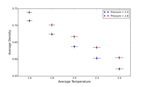
Theoretical results , based on the ideal gas law, give a higher density than the simulated result. (It can also be added that the discrepancy between the ideal and simulated systems increases with pressure.) It can be reasoned that the results provided by the Ideal Gas Law are higher due to the fact that particle-particle interactions are not consided.This means the repulsion that would be experienced by the particles moving closer to each other are not expressed, as such, particles the distance between particles can decrease without energyetic effects, thus increasing the density. Also Charles' law!

4 Calculation of heat capacities using statistical physics

4.1 Task

Run simulations and plot C_v/V as a function of temperature. Is this as expected?

Example input file: File:JmsD Cv 2.0 0.2.in

Example output file: File:JmsD Cv 2.0 0.2.log

For this section, 5 simulations were run for each of the two densities: 0.2, 0.8. These simulations corresponded to each of the respective temperatures: 2.0, 2.2, 2.4, 2.6, 2.8 (in reduced units). The desired results of these simulations were the calculated values of the Heat Capacity at constant volume, C_v. The results can be seen in Figure 4.1 as a funtion of the average temperatures.

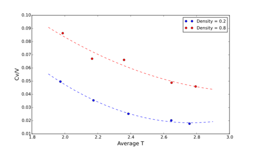
These graphs do indeed follow the trend expected, that is similar to the trend seen in a crystalline solid for example. The Heat Capacity is proportional to 1/T² [As seen in the Equations below] and as such a negative trend should be observed. Does it vary with the reciprocal of the square? Importantly, the variance in energy varies with temperature and therefore, we cannot take this argument. Think more either internal energies or density of states..

$C_{V} = \frac{\partial E}{\partial T} = N^{2} \frac{⟨ E^{2} ⟩ - {⟨ E ⟩}^{2}}{k_{B} T^{2}}$

With reagrds to density, C_v/V increases as the density increases - which is again as expected - because heat capacity is dependant on the amount of material per volume, and thus a denser material (with the same volume) has more mass or moles per unit voulume.

5 Radial Distribution Functions

5.1 Task

From simulations of the Lennard-Jones system in the three phases, Compute $g (r)$ and $\int g (r) d r$ in VMD. Discuss the differences in the 3 RDFs and thus what this means about the structure in each phase.

For the solid phase, illustrate which lattics sites the first 3 peaks correspond to. What is the Lattice spacing? What is the Coordination number for each of the first three peaks?

The initial parameters for the simulations, in order to specify the correct phases were:

Temperature: (For all phases) = 1.2 Densities: (Solid) = 1.50, (Liquid) = 0.85, (Vapour) = 0.01 Finally, to provide the initial positions of atoms, the simple cubic model was used for Liquid and Vapour, but for Solid FCC was used.

These parameters were calculated by examining the Lennar-Jones phase diagram found in literature. ^[2 ]

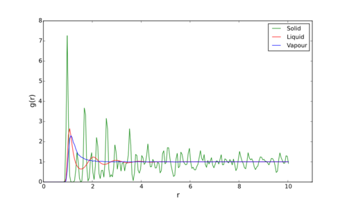
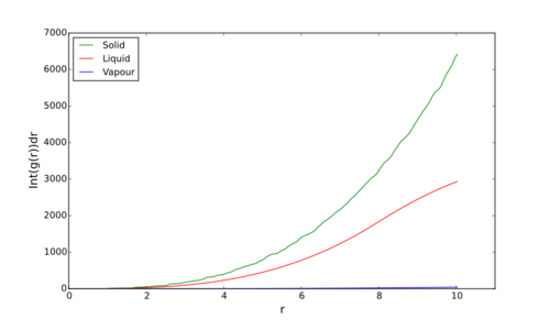
As it can be seen in Figure 5.1, the RDFs are very different for each phase. The area under the curves is the probability of finding another particle at that distance from the particle of reference, thus peaks are distances away from the reference that there is increased probability of encountering another.Tick for a normalised rdf

For example, the Vapour phase [as shown in blue in Figure 5.1] is largely simple. Whereas, the RDF of the liquid [purple] has a series of fairly ordered peaks of decresing height. This can be explained by the ease of motion of these two phases. Vapour particles are very spread out in space and have a lot more motion than liquids which are held together and inplace by various intermolecular/atomic bonds. Because of this by moving away fro a reference particle in the vapour phase, there is a very low probability of encountaring another particle. Liquids are a lot more ordered than gases and coordination spheres are shown by the fairly smooth peaks as r increases. There is reasonable probability of finsing another particle in the first coordination sphere, but this decreases as you move away further.Tick

Solids, on the other hand, have significantly greater order. The particles are generally held in a rather rigid lattice and their positions can be considered fairly fixed. In Figure 5.1 you can clearly see sharp peaks on the RDF as you move away from the reference, corresponding to neighbouring atoms. These come at regular distance intervals, which are the length of a unit cell away - This RDF in particular representing that of an FCC lattice. The area of these peaks does deacreas with distance somewhat as there is some movement, such as vibrations (especially if the particle's vibrations about the lattice point are coupled with vibrations of the lattice as a whole), that cause those further out to be proportionaly missalligned from their perfect lattice position.Tick, good explanation

6 Dynamical properties and the diffusion coefficient

6.1 Task

Run simlations for the three phases, to calculate the mean squared displacement and velocity autocorrelation functions.

Example input file:

File:JmsD.in

Example output file:

File:JmsD.log

6.2 Task

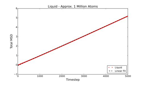
Measure D from it's connection to the MSD, for simulations and data for approx. one million atom simulations

These diff coeffs seem rather small.. Could be use of timestep?

The equation for the Diffusion Coefficient, $D = \frac{1}{6} \frac{\partial ⟨ r^{2} (t) ⟩}{\partial t}$ .

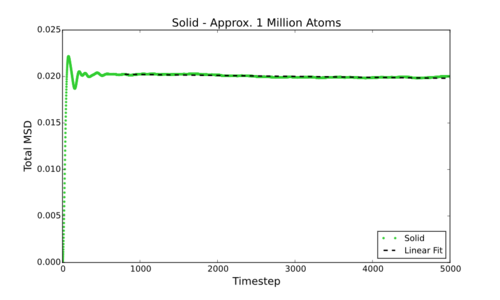
However, $D$ can be much more simply estimated by fitting the linear section of a Total MSD vs Timestep graph and dividing by 6. This gives the following values for D (in reduced units) for the smaller simulations carried out by myself:

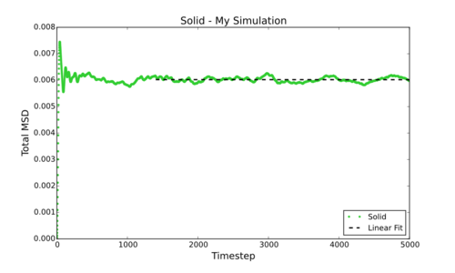
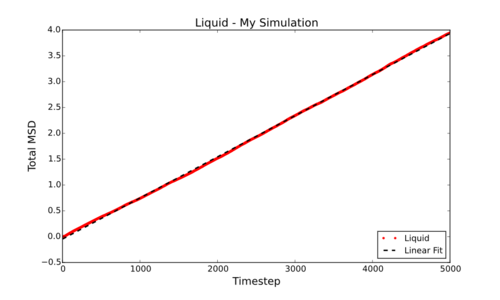
D_Solid = 1.31x10^-10 D_Liquid = 1.33^-4 D_Vapour = 1.55^-2 [The graphs for these calculations can be seen in Figures 6.1-6.3]

In comparison below are the values for D (in reduced units) for the larger (approx. 1 million atom) data supplied:

D_Solid = 1.71x10^-8 D_Liquid = 1.75^-4 D_Vapour = 6.28^-3 [The graphs for these calculations can be seen in Figures 6.4-6.6]

Tick

7 References

1.  LAMMPS Manual, http://lammps.sandia.gov/doc/Section_commands.html#lammps-input-script , accessed November 2016
2.  JP Hansen, L Verlet, Phys Rev, 184, 1969, http://journals.aps.org/pr/abstract/10.1103/PhysRev.184.151