Third year simulation experiment

Introduction to molecular dynamics simulation

Velocity Verlet Algorithm

What sort of a timestep do you need to use to ensure that the total energy does not change by more than 1% over the course of your "simulation"?

The initial total energy is 0.5, 1% change is between 0.495 and 0.505. 
After testing with different values of timestep, only the ones equal to or less than 0.2 fall in that range.

Why do you think it is important to monitor the total energy of a physical system when modelling its behaviour numerically?

First,we are simulating with classical particle approximation.
In the classical physical system, the potential energy and kinetic energy will interchange with each other,
i.e. the total energy is constant.
Also, we use statistical thermodynamics to calculate macroscopic properties from microscopic properties.
The simulation takes part in NVE ensemble if no ensemble is specified.
Thus in NVE ensemble the total energy does not change.
However, the total energy does fluctuates during the course of simulation due to the numerical approximation. 
The simulation is valid if the fluctuation falls in a small enough range (e.g.  $\pm 1 %$ )

Why do you think the error in the position changes with time in the way that it does?

Each new position is calculted using iteration, i.e. using the result from the previous calculation.
We will have error during mathematical approximation, and the error will be carried forward to the next position, 
resulting the increasing error in longer time.

Atomic Forces

For a single Lennard-Jones interaction, $ϕ (r) = 4 ϵ (\frac{σ^{12}}{r^{12}} - \frac{σ^{6}}{r^{6}})$ , find the separation, $r_{0}$ , at which the potential energy is zero.

As  $σ$  is the distance at which the  potential energy between the two particles is zero, 
the separation  $r_{0} = σ$  at which the potential energy is zero.

What is the force at this separation?

The Lennard-Jones force is  $F = - \frac{d ϕ}{d r} = \frac{24 ϵ}{r_{0}} [2 {(\frac{σ}{r_{0}})}^{13} - {(\frac{σ}{r_{0}})}^{7}]$ . When  $r_{0} = σ$ ,  $F = \frac{24 ϵ}{σ} (2 - 1) = \frac{24 ϵ}{σ}$ .

Find the equilibrium separation, $r_{e q}$ , and work out the well depth ( $ϕ (r_{e q})$ ).

At equilibrium separation,  $F = 0 = \frac{24 ϵ}{r_{0}} [2 {(\frac{σ}{r_{0}})}^{13} - {(\frac{σ}{r_{0}})}^{7}]$ . As  $σ$  and  $ϵ$  cannot be 0, thus  $r_{e q} = 2^{1 / 6} σ$ .
Substitute  $r_{e q} = 2^{1 / 6} σ$  into  $ϕ (r) = 4 ϵ (\frac{σ^{12}}{r^{12}} - \frac{σ^{6}}{r^{6}})$ , we can get  $ϕ (r_{e q}) = - ϵ$ .

Evaluate the integrals $\int_{2 σ}^{\infty} ϕ (r) d r$ , $\int_{2.5 σ}^{\infty} ϕ (r) d r$ , and $\int_{3 σ}^{\infty} ϕ (r) d r$ when $σ = ϵ = 1.0$ .

When  $σ = ϵ = 1.0$ ,  $ϕ (r) = 4 (\frac{1}{r^{12}} - \frac{1}{r^{6}})$ . 
Therefore  $\int ϕ (r) d r = 4 [(- \frac{1}{11} r^{- 11}) - (- \frac{1}{5} r^{- 5})] = - \frac{4}{11} r^{- 11} + \frac{4}{5} r^{- 5} + k$ .
Thus  $\int_{2 σ}^{\infty} ϕ (r) d r = 0 + \frac{4}{11} {(2 σ)}^{- 11} - \frac{4}{5} {(2 σ)}^{- 5} = \frac{1}{5632} σ^{- 11} - \frac{1}{40} σ^{- 5} = 1.78 σ^{- 11} - 2.5 * 1 0^{- 2} σ^{- 5}$ , 
      $\int_{2.5 σ}^{\infty} ϕ (r) d r = 0 + \frac{4}{11} {(2.5 σ)}^{- 11} - \frac{4}{5} {(2.5 σ)}^{- 5} = 1.52 * 1 0^{- 5} σ^{- 11} - 8.19 * 1 0^{- 3} σ^{- 5}$ ,
      $\int_{3 σ}^{\infty} ϕ (r) d r = 0 + \frac{4}{11} {(3 σ)}^{- 11} - \frac{4}{5} {(3 σ)}^{- 5} = 2.05 * 1 0^{- 6} σ^{- 11} - 3.29 * 1 0^{- 3} σ^{- 5}$ .

Periodic Boundary Conditions

Estimate the number of water molecules in 1ml of water under standard conditions. Estimate the volume of $10000$ water molecules under standard conditions.

 $1 m L * 1 g m L^{- 1} = 1 g$  water,  $1 g / 18 g m o l^{- 1} = \frac{1}{18} m o l$  water,  $\frac{1}{18} m o l * 6.02 * 1 0^{23} m o l^{- 1} = 3.35 * 1 0^{22}$  molecules of water.
 $10000 / 6.02 * 1 0^{23} m o l^{- 1} = 1.66 * 1 0^{- 20} m o l$  of water,  $1.66 * 1 0^{- 20} m o l * 18 g m o l^{- 1} = 2.99 * 1 0^{- 19} g$  water  $= 2.99 * 1 0^{- 19} m L$  water.

Consider an atom at position $(0.5, 0.5, 0.5)$ in a cubic simulation box which runs from $(0, 0, 0)$ to $(1, 1, 1)$ . In a single timestep, it moves along the vector $(0.7, 0.6, 0.2)$ . At what point does it end up, after the periodic boundary conditions have been applied?

As the direction of moving is  $(0.7, 0.6, 0.2)$ , the x-direction moves the fastest and will reach the boundary first.
The time  $t$  required for the atom to move to the boundary can therefore be expressed as  $0.5 + 0.7 t = 1.0$  where  $t = 0.7$ .
Thus at  $t = 0.7$ , the duplicate atom will enter the central box at  $(0.0, 0.9, 0.6)$ .

Reduced Units

The Lennard-Jones parameters for argon are $σ = 0.34 n m, ϵ / k_{B} = 120 K$ . If the LJ cutoff is $r^{*} = 3.2$ , what is it in real units? What is the well depth in ${k J m o l}^{- 1}$ ? What is the reduced temperature $T^{*} = 1.5$ in real units?

Distance  $r = σ * r^{*} = 0.34 n m * 3.2 = 1.09 n m$ .
Well depth is equal to  $- ϵ$ , thus  $E = ϵ * E^{*} = 0.997 {k J m o l}^{- 1} * (- 0.997) = - 0.994 {k J m o l}^{- 1}$ 
Temperature  $T = T^{*} * (ϵ / k_{B}) = 1.5 * 120 K = 180 K$ .

Equilibration

Creating the simulation box

Why do you think giving atoms random starting coordinates causes problems in simulations?

If the atoms are giving randon initial positions, some of them might turn out to be too close from each other (distance smaller than ).
They will repel each other until they are enough far apart, which results in release of plenty of potential energy to stablise.
This potential energy then changes to kinetic energy and heat the whole system up which is undesirable.

Satisfy yourself that this lattice spacing corresponds to a number density of lattice points of 0.8. Consider instead a face-centred cubic lattice with a lattice point number density of 1.2. What is the side length of the cubic unit cell?

Number density equals number of lattice points per unit volume and the number of lattice point of primitive cubic system is 1,
therefore unit volume=number of lattice points/number density=1/0.8=1.25. 
Lattice spacing=(unit volume)^1/3=1.0772.

For face-centred cubic lattice, the number of lattice point of a unit cell is 4.Therefore unit volume=4/1.2=3.33.
Lattice spacing=(unit volume)^1/3=1.4933.

Consider again the face-centred cubic lattice from the previous task. How many atoms would be created by the create_atoms command if you had defined that lattice instead?

Number of unit cells is 1000 (10*10*10) and 4 lattice points per unit cell, therefore 4000 atoms on the 4000 lattice points of 1000 unit cells.

Setting the properties of the atoms

Using the LAMMPS manual, find the purpose of the following commands in the input script:

mass 1 1.0
The mass command has syntax as mass I value^[1] where I is the atom type and value is the mass of the atom in reduced units.
The mass can be set for one or more atom type, by just numbering or using * as wild-card.

pair_style lj/cut 3.0
The pair_style command has syntax as pair_style style args^[2]. There are plenty of styles describing the interaction between two atoms.
As we are modelling the interaction pairs of atoms in simple liquid, we just use Lennard-Jones potential to calculate the interaction, i.e. using pair_style lj/cut command.
The cut in args means 'cutoff' distance, which means that any pair interaction are ignored if their distance is beyond 'cutoff' distance (3.0 in this case).
Also the 'cutoff' distance must be smaller than half of the box length or some same interactions would be taken into account twice.

pair_coeff * * 1.0 1.0
The pair_coeff command has syntax as pair_coeff I J args^[3] and are used to define coefficients after pair_style lj/cut command $σ = ϵ = 1.0$  in this case^[4].
I,J are the type of atoms that are interacting with each other, and two single asterisk (* *) means that both interacting atom can be chosen from all atoms.
1.0 1.0 is the args, which means  $σ = ϵ = 1.0$  in this case^[4].

Given that we are specifying $x_{i} (0)$ and $v_{i} (0)$ , which integration algorithm are we going to use?

We are going to use Velocity Verlet Algorithm.

Running the simulation

Look at the lines below.

### SPECIFY TIMESTEP ###
variable timestep equal 0.001
variable n_steps equal floor(100/${timestep})
variable n_steps equal floor(100/0.001)
timestep ${timestep}
timestep 0.001

### RUN SIMULATION ###
run ${n_steps}
run 100000

The second line (starting "variable timestep...") tells LAMMPS that if it encounters the text ${timestep} on a subsequent line, it should replace it by the value given. In this case, the value ${timestep} is always replaced by 0.001. In light of this, what do you think the purpose of these lines is? Why not just write:

timestep 0.001
run 100000

The lines below ### SPECIFY TIMESTEP ### tells the software that the timestep equal 0.001 per step, the simulation time is 100, and thus there are 100000 steps to run. 
As we need to compare the results with same simulation time, therefore if we change timestep to 0.002 per step and just write run 100000,
we will end up with a simulation of  $0.002 * 100000 = 200$  steps which we do not want.
If we use lines below ### SPECIFY TIMESTEP ###, we will result in simulation time of 100 whatever timestep we choose.

Checking equilibration

Make plots of the energy, temperature, and pressure, against time for the 0.001 timestep experiment (attach a picture to your report). Does the simulation reach equilibrium? How long does this take?

The simulation reaches the equilibrium.
It takes about 0.25 to reach equilibrium.

When you have done this, make a single plot which shows the energy versus time for all of the timesteps Choosing a timestep is a balancing act: the shorter the timestep, the more accurately the results of your simulation will reflect the physical reality; short timesteps, however, mean that the same number of simulation steps cover a shorter amount of actual time, and this is very unhelpful if the process you want to study requires observation over a long time. Of the five timesteps that you used, which is the largest to give acceptable results? Which one of the five is a particularly bad choice? Why?

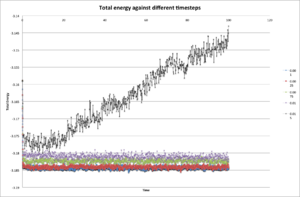
Timestep of 0.0025 is the largest to give
acceptable results as it almost provides
the same result as the timestep of 0.0001
during course of approximation.
However, if using both timesteps to simulate
same number of steps, timestep of 0.0025
will have 2.5 times more of actual simulation
time, and is desirable for long time simulation.

Running simulations under specific conditions

Temperature and Pressure Control

Choose 5 temperatures and two pressures . This gives ten phase points — five temperatures at each pressure. Create 10 copies of npt.in, and modify each to run a simulation at one of your chosen $(p, T)$ points. You should be able to use the results of the previous section to choose a timestep.

The five temperatures are 1.6, 1.8, 2.0, 2.2, 2.4 and the two pressures are 2.4 and 2.6. The timestep chosen is 0.0025.

Thermostats and Barostats

We need to choose $γ$ so that the temperature is correct $T = 𝔗$ if we multiply every velocity $γ$ . We can write two equations:

$\frac{1}{2} \sum_{i} m_{i} v_{i}^{2} = \frac{3}{2} N k_{B} T$ (1)

$\frac{1}{2} \sum_{i} m_{i} {(γ v_{i})}^{2} = \frac{3}{2} N k_{B} 𝔗$ (2)

Solve these to determine $γ$ .

 $\frac{1}{2} \sum_{i} m_{i} {(γ v_{i})}^{2} = \frac{3}{2} N k_{B} 𝔗 = \frac{1}{2} γ^{2} \sum_{i} m_{i} v_{i}^{2} = \frac{3}{2} N k_{B} 𝔗$  (3)
(3) divided by (1) results in  $γ^{2} = \frac{𝔗}{T}$  and  $γ = \sqrt{\frac{𝔗}{T}}$ .

Examining the Input Script

Use the manual page to find out the importance of the three numbers 100 1000 100000. How often will values of the temperature, etc., be sampled for the average? How many measurements contribute to the average? Looking to the following line, how much time will you simulate?

100 is Nevery = use input values every this many timesteps; 1000 is Nrepeat = # of times to use input values for calculating averages;
100000 is Nfreq = calculate averages every this many timesteps^[5].
In this case, the software calculate and display the temperature, etc. after 100000 timesteps (i.e. only at the end of the simulation), 
the average thermodynamic properties are calculated from 1000 inputs, which are taken every 100 timesteps (the 100th, the 200th, the 300th, etc.).

Plotting the Equations of State

Use software of your choice to plot the density as a function of temperature for both of the pressures that you simulated. Your graph(s) should include error bars in both the x and y directions. You should also include a line corresponding to the density predicted by the ideal gas law at that pressure. Is your simulated density lower or higher? Justify this. Does the discrepancy increase or decrease with pressure?


Plot of density vs. temperature at p=2.4 and 2.6 with error bar in both x and y directions.	Plot of density vs. temperature at p=2.4 and 2.6 with comparison with density calculated from ideal gas law

The density is calculated from ideal gas law in this way,
 $p V = n R T$ , as  $n = N * N_{A}$ , thus  $p V = N * N_{A} R T$ .
As $N_{A} * R = k_{B}$ , thus  $p V = N k_{B} T$ .
Therefore,  $ρ = \frac{N}{V} = \frac{p}{k_{B} T} = \frac{p}{T}$  as  $k_{B} = 1$  in reduced unit.
Both simulated densities at different pressures are lower than calculated from ideal gas law. 
The densities are simulated with temperature above the critical temperature, thus the atoms are in fluid state.
The properties at fluid state are better described by Van der Waals equation instead of the ideal gas law^[6].
The ideal gas law is more validate to the real situation at high temperature and low pressure.
The discrepancy of density on the plot decrease as temperature increases and pressure decreases,
which agrees with the validate condition of ideal gas law.

Calculating heat capacities using statistical physics

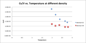
As in the last section, you need to run simulations at ten phase points. In this section, we will be in density-temperature $(ρ^{*}, T^{*})$ phase space, rather than pressure-temperature phase space. The two densities required at $0.2$ and $0.8$ , and the temperature range is $2.0, 2.2, 2.4, 2.6, 2.8$ . Plot $C_{V} / V$ as a function of temperature, where $V$ is the volume of the simulation cell, for both of your densities (on the same graph). Is the trend the one you would expect? Attach an example of one of your input scripts to your report.

Input script with T=2.0, ρ=0.2 here.
The trend showing that there is inverse correlation between Cv/V and density,
increasing temperature causing decreasing Cv/V both agree with real condition.

Structural properties and the radial distribution function

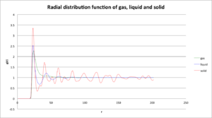
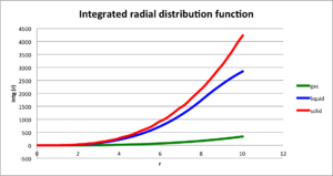
Plot the RDFs for the three systems on the same axes, and attach a copy to your report. Discuss qualitatively the differences between the three RDFs, and what this tells you about the structure of the system in each phase. In the solid case, illustrate which lattice sites the first three peaks correspond to. What is the lattice spacing? What is the coordination number for each of the first three peaks?

The rdf of solid is continuous array of sharp spikes but decreasing with increasing r.
This sharp spikes suggests that most particles lie in definite locations with only small oscillation.
The rdf of liquid is more smooth,with only two slightly sharper peak, meaning less ordered structure.
The particles closer to the target particle may still adopt the their initial position while the further particles clear do not,
which the probability of finding a particle in different places of long distance is all equal.
The rdf of gas only has one sharp peak, which is the position with lowest Lennard-Jones potential,
where particles are more likely to stay, also the probability of finding particles in other places further than that is all the same.

In the solid case, illustrate which lattice sites the first three peaks correspond to. What is the lattice spacing? What is the coordination number for each of the first three peaks?

The first three peaks correspond to face-centered-cubic structure.
In solid, the first three peaks have [r,g(r)] as [1.075,3.347],[1.575,0.617] [1.925,1.720], 
the output file shows the lattice spacing r is1.5874 is close to the r of the second peak (r₂ ).
First peak at r₁ has approximate value of  $r_{2} / \sqrt{2}$ ,
third peak at r₃ has approximate value of  $r_{2} * \sqrt{2}$ .
Therefore, in a cubic, if the position of reference particle is at (0,0,0),
then particles with distance r₁ has relative position (0.5,0.5,0) and coordination number is 12;
particles with distance r₂ has relative position (1,0,0) and the coordination number is 6;
particles with distance r₃ has relative position (1,0,1) and the coordination number is 12.


Radial distribution function of gas, liquid and solid.	Integrated radial distribution function of gas, liquid and solid.

Dynamical properties and the diffusion coefficient

Mean Squared Displacement

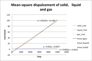
Make a plot for each of your simulations (solid, liquid, and gas), showing the mean squared displacement (the "total" MSD) as a function of timestep. Are these as you would expect? Estimate $D$ in each case. Be careful with the units! Repeat this procedure for the MSD data that you were given from the one million atom simulations.


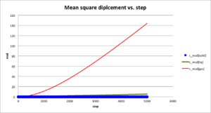Mean square displacement vs. step of gas, liquid and solid.	Mean square displacement vs. step of gas, liquid and solid with one million atoms.

The msd plot agrees with the realistic condition.
The general trend of msd is gas>liquid>solid and msd of gas increases much more with time than other two.
Solid and liquid diffuse less than gas from initial position during the same period of time due to their strong intermolecular force.
The gradient msd of each state is shown in plot above. 
For gas,  $D = \frac{1}{6} \frac{\partial ⟨ r^{2} (t) ⟩}{\partial t} = \frac{1}{6} * 0.0222 = 3.7 * 1 0^{- 3}$ ;
for liquid,  $D = \frac{1}{6} * 0.001 = 1.7 * 1 0^{- 4}$ ;
for solid,   $D = \frac{1}{6} * 0.0003 = 5.0 * 1 0^{- 5}$ .

Velocity Autocorrelation Function

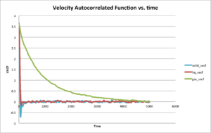
In the theoretical section at the beginning, the equation for the evolution of the position of a 1D harmonic oscillator as a function of time was given. Using this, evaluate the normalised velocity autocorrelation function for a 1D harmonic oscillator (it is analytic!): $C (τ) = \frac{\int_{- \infty}^{\infty} v (t) v (t + τ) d t}{\int_{- \infty}^{\infty} v^{2} (t) d t}$

 $v (t) = \frac{d x}{d t} = - A ω s i n (ω t + ϕ)$

Be sure to show your working in your writeup. On the same graph, with x range 0 to 500, plot $C (τ)$ with $ω = 1 / 2 π$ and the VACFs from your liquid and solid simulations. What do the minima in the VACFs for the liquid and solid system represent? Discuss the origin of the differences between the liquid and solid VACFs. The harmonic oscillator VACF is very different to the Lennard Jones solid and liquid. Why is this? Attach a copy of your plot to your writeup.

Use the trapezium rule to approximate the integral under the velocity autocorrelation function for the solid, liquid, and gas, and use these values to estimate $D$ in each case. You should make a plot of the running integral in each case. Are they as you expect? Repeat this procedure for the VACF data that you were given from the one million atom simulations. What do you think is the largest source of error in your estimates of D from the VACF?

The trapezium rule is  $\int_{0}^{5000} f (x) d x = \frac{1}{2} h [(y_{0} + y_{5000}) + 2 (y_{1} + y_{2} + y_{4999})]$ ,  $h = (x_{n} - x_{0}) / n$ .
For solid, integration equals to 26.96, for liquid, integration equals to 146.83, integration equals to 3204.02.

References and citations

↑ http://lammps.sandia.gov/doc/mass.html
↑ http://lammps.sandia.gov/doc/pair_style.html
↑ http://lammps.sandia.gov/doc/pair_coeff.html
↑ ^4.0 ^4.1 http://lammps.sandia.gov/doc/pair_lj.html
↑ http://lammps.sandia.gov/doc/fix_ave_time.html
↑ TL Hill; Introduction to Statistical Thermodynamics. Addison-Wesley, Reading (1960) p280

[mass_command-1] ttp://lammps.sandia.gov/doc/mass.html

[pair_style_command-2] ttp://lammps.sandia.gov/doc/pair_style.html

[pair_coeff_command-3] ttp://lammps.sandia.gov/doc/pair_coeff.html

[pair_style_args-4] 4.0 ^4.1 http://lammps.sandia.gov/doc/pair_lj.html

[average-5] ttp://lammps.sandia.gov/doc/fix_ave_time.html

[VDW_equation-6] TL Hill; Introduction to Statistical Thermodynamics. Addison-Wesley, Reading (1960) p280

[1]

[2]

[3]

[4]

[5]

[6]