In Inorganic Chemistry the bonding and the structure of inorganic materials such as transitional metal complexes can be investigated using computational as opposed to experimental techniques. These computational methods allow for a more detailed look at what is actually occurring between two atoms when a bond is formed. Computational methods gives a method of being able to highlight stable conformers of a molecule and further even identify transition states, in turn this allows for quantitative representations of the various energy gaps.
Creating and Optimising a Molecule
The program Gaussian was used in order to carry out the different elements of the computational investigation. A BH3 molecule was created in the Gaussview interface, in the following way. The periodic table tab was opened and the boron element was selected, the planar fragment was then selected. Once the molecule had been created the different controls were explored in order to manipulate the molecule ie;
BH3
rotating the molecule
magnifying and decreasing the size of the molecule
translating the molecule
The bond distances and bond angles were also observed using the related Gaussview functions.
The optimisation of BH3 was then carried out. The optimisation is a two part process where for the electron density and the energy in BH3 Schrodinger's equation is solved. Then the nuclei wihtin the molecule are moved in order to find the ideal position at which the energy of the conformer is at its minimum. The calculation was completed with the following constraints:
Method: B3LYP
Basis Set: 3-21G
Type of Calculation: OPT for an optimisation
Each constraint informs the program of the type of calculation that is required for the optimisation. The method used is the one that is utilised by the system to make the particular approximation/calculation. The basis set denotes the level of accuracy for the calculation and for borane this was set to 3-21G which is a fairly low level of accuracy. This low level of accuracy was chosen in order to ensure that the calculation was completed quickly. Once the BH3 molecule had been optimised by Gaussian the molecule could then be viewed using the Gaussview interface.
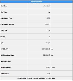
The particulars of the optimised molecule can be found in the results summary shown.BH3 Summary The summary shows the type of file, the method and the basis set all of which were already known prior to the optimisation, however the summary also produces information about the quantitive energy. The energy for the optimised BH3 was -26.46226433 a.u. the energy is given in atomic units which is actually Hartree. It can be noted also that the energy of the molecule is negative this too could allude to the fact that the optimisation has found an optimised structure with a minimum energy. If the units are converted into kcal mol-1 one can get a more useful picture of the optimised molecule. The summary also shows the length of the calculation. If this initial time was very long it would be advised to continue the calculations on the SCAN system that uses the cpu processing of several machines as opposed to one. The summary file also gave the point group of the borane molecule as D3h this is the correct point group for the trigonal planar borane structure which has identical hydrogens.
Graphs plotting the optimisation step number against the total energy and the RMS gradient were obtained. The gradient is key in informing one whether the optimisation has actually been successful. If the gradient is significantly close to zero ie; less than the value of 0.001 then one can be almost certain that the molecule has been fully optimised.
Total Energy against the Optimisation Step NumberRMS Gradient against the Optimisation Step Number
When the molecule undergoes optimisation the system is solving Schrodinger's equation for a series of positions of the nuclei and the electrons. This is then repeated and in this way the program attempts to find the best configuration/co ordinates of the said nuclei and electrons for the particular basis set denoted. By analysing the graphs one can count the exact number of iterations that were required to minimise the gradient and obtain the optimum structure.
Another way to check that the molecule has been optimised, which is not a graphical method, is by reading the *log.file created by the program upon optimisation. By looking at the last set of forces and displacements and seeing whether the calculation has converged. If the forces have indeed converged it means that for very small alterations of the forces the energy has not altered leading to that fact that the optimised molecule has been found.
Molecular Orbitals of BH3
A useful feature of computational chemistry methods is the ability to produce visual tools to aid understanding of the bonding within inorganic molecules. Representations of the molecular orbitals in the trigonal planer BH3 molecule were computed and then compared with the molecular orbitals derived using LCAO (Linear Combination of Atomic Orbital) Theory. The checkpoint file (*.fchk) from the optimised BH3 WAS downloaded from the scan system and the calculation required to obtain the molecular orbitals and full natural bonding orbitals was also selected to be calculated. Once put into the Gaussview calculation tab the calculation reads:
# b3lyp/3-21g pop=(full) geom=connectivity
BH3
The Molecular Orbital file of BH3 can be found here: Molecular Orbitals of BH3 Below the derived molecular orbitals of BH3 have been depicted. The 1s atomic orbital of boron has not been depicted and this is because the atomic orbital lies significantly deep enough not to be involved in the bonding between the boron and the hydrogen atoms. However one should note that in Inorganic chemistry generally all the molecular orbitals are considered to fully understand the manner in which the atoms and overall the molecule is bonded. As mentioned however the atomic orbital has not been fully considered due to the fact that in this simplified model it does not directly contribute to the molecular bonding.
The two sets of Molecular Orbitals can now be compared alongside each other in more depth.
Table showing comparison between the computed MOs and the LCAO MOs
LCAO derived Molecular Orbitals
Computed/real Molecular Orbitals
Description
1a1'
HOMO-3
The computed molecular orbital for the 1s B fragment is very similar to the one derived using LCAO method. The 'real' method gives a three dimensional representation of the spherical electron distribution/density.
2a1'
HOMO-2
The computed moleuclar orbital gives a more distributed picture of the electron density. Whereas, although similar, the derived molecular orbitals give specific and defined areas where the electron density is located.
1e'
HOMO
The computed MO is very clear in its representation of a nodal plane where there is no electron density. However the derived MO show the in phases and out of phase nature of the MO with the relative proportions of the s and p orbitals.
1e'
HOMO-1
The derived LCAO orbitals are able to show the interactions between the atomic orbitals to achieve an overall bonding interaction well. The computed MOs have blended the regions of electron density and also shows regions in the molecule with electron deficiency much better.
1a2
LUMO
The derived MOs show positioning of the electron density as central of the molecule therefore its mainly centred on the boron atom. The computed MOs however show the molecular orbitals to be covering the whole molecule.
3a1'
LUMO+1
Both methods provided very similar depictions of the molecular orbitals and they also showed the anti-bonding nature of the orbitals well.
2e'
HOMO+3
These orbitals depicted are strongly anti-bonding adn the computed MOs actually shows the distortion of one of the B p orbitals as the orbital tries to minimise its energy. The LCAO MOs are not able to take into account the adjustment of the orbitals.
2e'
LUMO+2
The derived MOs although show all the elements that contribute to the MO, are not able to blend these contributions together giving a slightly disjointed depiction of the MO. The computational method however provides a clear visual three dimensional description of the MO and the manner in which the different contributions from the different atomic orbitals to give a fairly accurate MO.
Overall both methods provided a very clear depiction of the molecular orbitals of the BH3 molecule. The Linear Combination of Atomic Orbital method gives a clear picture of the relative contributions. The computational method however allows for a three dimensional graphical representation of the molecular orbitals, the computational generated MOs also show how the orbitals blend and how the orbitals distort to attempt to stabilise the molecule as much as possible. Although visually the computational method appears superior the LCAO method allows for a quick representation and also proves that the computer calculations are correct.
NBO analysis of BH3
By carrying out an NBO calculation on the said molecule the nature of the charges and how this affects the structure of the molecule can be further explored. By colouring the hydrogens and the boron a different colour one can see the difference in the charges explicitly. The program also shows density of the charges, the more vivid the colours on the different atoms the more localised the charge. The fact that the boron bright vivid green indicates that it is highly positively charged and the converse is true for the brightness on the hydrogens. One should also remember that the idea of the boron being highly positively charged and the hydrogens being significantly negatively charged is relative and for this molecule calculated,it would not be accurate to use the brightness of the charged atoms as a universal scale. By looking at the actual values that were calculated by the system one can see that they too correspond with the coloured depiction. The NBO value for Hydrogen was -0.09 and for the Boron 0.28, one coudl say that the hydrogens therefore have more electron density whereas boron is more electron deficient. This depiction of boron is reflected in its actual chemistry where it happily forms adducts as a Lewis when coordinated to 3 other atoms.
Atoms coloured by chargeAtomic charges
Frequency and IR analysis of BH3
The frequency calculation was very similar to that for the obtaining of the molecular orbitals however on the first attempt of retrieving the output file after the calculation the logfile (*.log) appeared empty, and so the molecule of BH3 was unable to be opened. Prior to the frequency calculation the optimised file had been saved so the process was repeated and a title was put into the file and the intermediate geometries were un-checked, there is a chance that this was the reason the previous calculation was unsuccessful. Once the succesful output file was opened the various vibrations were analysed and the readable log file was checked to ensure the calculation had converge and there were no errors. No negative frequencies were observed meaning that the molecule had been optimised to the best of the programs capabilities. Teh low frequencie sin the logfile were also noted as being significantly close to 0 also providing more evidence that the frequency calculation had been carried out on the correct molecule.
Vibrational Analysis Table
Vibration No.
Pictoral depiction of the Vibration
Frequency cm-1
Intensity
Symmetry D3h Point Group
1
1146.03
92.66
A2
2
1204.86
12.39
E'
3
1204.86
12.39
E'
4
2591.65
0.00
A1'
5
2730.07
103.86
E'
6
2730.07
103.86
E'
The IR spectrum was also obtained:
A total of 6 vibrations were provided by the system this is in-keeping with the idea of there being 3n-6 vibrational frequencies. Teh IR spectrum however only shows a total of 3 peaks. The fourth vibration has A1' symmetry this means that all elements are symmetrical including its vibrations therefore the vibrations cancel out and there is no overall peak detected meaning it is in fact IR in-active. There are also two pairs of degenerate vibrations whic have identical intensities and frequencies. These however are IR active but correspond to the same values. Overall this gives 3 peaks as observed in the IR spectrum obtained. When these frequencies were compared with those in the literature one can see that the literature values of 1125cm-1, 1640cm-1 and 2808cm-1[1]. The discrepancies between the literature and the computational methods show that the calculation provided over-estimates of the frequencies, meaning the calculation leads one to believe that the bonds are stronger than they actually are.
Optimisation and Analysis of TlBr3
The TlBr3 molecule was optimised and analysed in a similar manner to BH3 the calculation constraints were set as follows:
Method: B3LYP
Basis Set: LanL2DZ
Type of Calculation: OPT for an optimisation
As one can see the basis set used for TlBr3 and BH3 were different although the method was kept the same. This is due to the fact that Thallium is significantly larger than Bromine and in order to ensure that the calculation was as accurate as possible are more detailed basis set was used. This allows for the extra orbitals that are part of larger atoms to be accurately represented and considered in the calculations. Another difference between this calculation was that the symmetry of the molecule was restricted to the D3h point group, once again down to the size of the Thallium and the fact that it also resides very close to the transition metals in the periodic table meaning that it may behave in a similar manner and be more than 3 coordinate depending on the substituents.
The optimisation adn the frequency analysis of the molecule were carried out using hte same basis set and the same method to ensure that the same orbitals were considered when optimising and calculating the frequencies. On optimisation the bond distance and bond angles are shown in the pictures below:
Bond DistanceBond Angle
The bond distance and bond angles should be read accurate to two decimal places as the calculation is an approximation in itself and is not fully accurate. TheOptimisation of Thallium Bromide was only deemed accurate once the frequency calculation had been done, once the frequency and molecular orbital calculation, which was done simultaneously in order to save time, the logfile was checked to see whether the low frequencies were close enough to zero to be sure that a minimum conformer had been found. TheMolecular Orbitals of Thallium Bromide were deemed to have been done on the optimised structure. The bond distance obtained using the computational method was 2.65Å and the bond length in the literature was 2.52Å[2] one can see that the computational method actually gave a value very close to that in the literature. The value however was an overestimate. In order to increase the accuracy further the basis set could be altered to a more accurate one. However this value was significantly better than the bond distance obtained after a 3-21G optimisation (2.68Å). This again helos to prove that the better the basis set the more accurate the results obtained by the computational method. Fot eh thallium structure the bonds were drawn and visible in Gaussview however in the Molybdenum structure this was not the case and it shall be discussed in the next section.
Investigating Cis and Trans Isomerism in Molybdenum octahedral Complexes
For this particular investigation the structural features of two octahedral Mo(CO)4L2 complexes were investigated using vibrational analysis and other spectral tools. The two structures can be be viewed and are formed either by the L ligands adopting axial (trans) positioning or alongside each other (cis), for the purpose of the investigation PCl3 was set as the L ligand as the initial suggested PPh3 will have required a substantial amount of computational time and power.
Cis-Mo(CO)4(PCl3)2Trans-Mo(CO)4(PCl3)2
The molecules were drawn using Gaussview and optimised in the same fashion. However due to the complex nature of the structure the constraints used were:
Method: B3LYP
Basis Set: LANL2MB
Calculation: OPT for a optimisation opt=loose to ensure it converged
Initially when the calculation was complete the new optmised molecules had the bonds between the Mo and the P missing these are the structures shown in the 3D jmols above. The bonds aree not shown because the distances calculated were deemed too long for a bond to actually be depicted by the system, in general Gaussview is known to recognise organic molecules which generally have much shorter bonds. The initial optimisation just provides a starting point for the optimisation of the isomers. Having optimised these structures initially they were then manually altered using the rotation tools. The cis isomer was altered so that one of the PCl3 ligands had a dihedral angle of 0o the trans isomer was manually altered so that both of the PCl3 were eclipsed, the dihedral angles for both of the ligands was set to 0o in accordance with CO ligands. These alterations were made to find a conformer for the two that was even lower in energy, the RMS gradient on completion was however still quite small meaning that basis set's accuracy and the geometry of the initial molecules made it difficult to find the energy minima straight away. The new constraints were:
Method: B3LYP
Basis Set: LANL2DZ
Calculation: OPT for a optimisation "int=ultrafine scf=conver=9" to increase electronic convergence.
The files for the second optimisation can be found here: Cis-Mo(CO)4(PCl3)2 and Trans-Mo(CO)4(PCl3)2 The pseudo potential and basis set were changed in order to obtain more accurate representations of the optimised molecules. Combining the manual alteration of their geometries and the more sophisticated basis set the calculation took relative less time. In order to ensure that the correct optimised molecules were produced the logfile and the frequencies had to be checked. Because the obtained structures all contained positive frequency values one could conclude that the correct molecules had been optimised. The optimised structures can be viewed below along with the appropriate information concerned or provided by the calculation. The files can be found here: Vibrational Calculation Cis and Vibrational Calculation Trans.
Table 1
Trans-complex
File Type
.log
Calculation Type
FOPT
Calculation Method
RB3LYP
Basis Set
LANL2DZ
Charge
0
Spin
Singlet
E(RB3LYP)
-623.57603100 a.u.
RMS Gradient Norm
0.00003121 a.u.
Imaginary Freq
Dipole Moment
0.3048 Debye
Point Group
C1
Table 2
Cis-complex
File Type
.log
Calculation Type
FOPT
Calculation Method
RB3LYP
Basis Set
LANL2DZ
Charge
0
Spin
Singlet
E(RB3LYP)
-623.57707196 a.u.
RMS Gradient Norm
0.00000259 a.u.
Imaginary Freq
Dipole Moment
1.3101 Debye
Point Group
C1
The relative Energies of the Cia and Trans Isomers
Isomer
Energy / a.u.
Energy / kJmol-1
cis
-623.58
-1637201.73
trans
-623.58
-1637198.99
Energy Difference
0.00
2.73
The above table provides the relative energies of the two isomers one can see the energy values in atomic units, Hartree, as given by the system and kJmol-1 which is a more qualitative. The cis isomer was the isomer deemed most stable after the calculations as it had a more negative energy value. If one relied on Hartree to report the energies the two isomers could be mistaken to have the same energy however on conversion to kJmol-1 one can see that there was a small difference that was then detected. Initially it could be assumed that the trans isomer would be more stable just by looking at the structures as the PCl3 ligands are as far apart as possible reducing the likelihood of steric clash especially as they are significantly larger ligands than the carbonyl ones. It is possible that the basis set was not detailed enough to provide the trans molecule with the lowest energy. If the PPh3 ligands had been used it would most likely have produced the trans isomer with the lowest energy as the ligands are substantially large and sterically bulky.
Vibrational Analysis of Cis and Trans Molybdenum octahedral Complexes
As the vibrations were checked to ensure that their frequencies were all positive these could then be analysed to provide further information about their geometries. The vibrations shown in the table are as a result of vibrations along the molybdenum-phosphorous bond. As the temperature is increased as will the thermal energy therefore one can also assume that the vibrations also increase with increasing temperature.
Table showing the Low Energy Vibrations of cis- and trans- Mo(CO)4(PCl3)2
Isomer
Vibration
Frequency / cm-1
cis
10.73
trans
5.04
trans
6.05
In total there were 4 carbonyl stretches that were calculated and this coincides with the number of ligands that were present. In the trans complex fewer stretches were reported and this could be due to the high symmetrical nature of the isomer. The trans isomers also had two stretches that were computed to have extremely low intensities. In the IR spectra for the cis complex there were distinct peaks mapping onto the 4 distinct C-O ligands present in the isomer as each C-O could be said to be in a chemically distinct environment. The trans complexes IR however only had two visible peaks of high intensity and these are the ones that were not cancelled out due to symmetry.
Analysis of the Structures of cis- and trans-Mo(CO)4(PCl3)2
Below is a table that compares the geometrical parameters of the complexes calculated to those stated in the literature [3].
Mo-P Bond Length Â
Mo-C Bond Length Â
C-O Bond Length Â
P-Mo-P Bond Angleo
P-Mo-C Bond Angleo
C-Mo-C Bond Angleo
Literature Value
2.50
2.01
1.65
180
87.2
180
Computed Value
2.44
2.06
1.17
177
91
179
The calculated values and those found in the literature can be seen to coincide considering that the computational method relies on multiple approximations. The values are all of the same order of magnitude which once again shows the power of having the ability to use computational methods in order to further explore the structure of inorganic compounds.
Inorganic Mini-Project
Investigating the Structure and Bonding in Select Ionic Liquids
Objective
Ionic liquids are solvents used in electrochemical reactions, they are salts which due to the lack of coordination are liquids below 100oC some of these salts are even liquid at room temperature (these are known as RTIL's-Room Temperature Ionic Liquids). Generally one of the atoms is organic and an ion also has a delocalised charge combined this factors prevent the salt from forming a more stable lattice crystal structure. The pyridinium ion was seen as a good starting point for the formation of ionic liquids. The properties of the liquid such as the viscosity, melting points and solubilities vary on the altering of the substituents on the organic group as well as the counter-ion used to stabilise the delocalised charge. This means that ionic liquids can be made to meet specific requirements for individual reactions making them extremely useful synthetic compounds.
In order to investigate the structure and nature of the bonding in ionic liquids several molecules were chosen: two pairs with identical Group 15(V) positive ions.
Optimisaations
Summary of properties for Ionic Liquids investigated
Ionic Liquid
Bond Length
Bond Angle
PMe3H+
1.866
111.217
PCl3H+
2.146
110.667
NMe3H+
1.532
110.995
NCl3H+
1.852
111.786
From the table of properties one can see that the the larger the the group 15 ion the longer the bond is between the central ion and the susbstituents. The phosphorous molecules in general had longer bonds than the nitrogen containing molecules. On changing of the substituents from methyl groups to chlorine atoms for both pairs of molecules the bond length increases by the same qualitative amount.
The molecules were optimised using the same method and calculated in the same manner that was discussed at the start of the project with the following becoming the new constraints:
Method: B3LYP
Basis Set: 6311G (d,p)
Type of Calculation: OPT for an optimisation
The method was the same as utilised throughout the exercise however the molecules were first optimised using the small 3-21G basis set. The basis set was then increased to the more accurate 6311G basis set. Because this method is more accurate it was expected to take a lot more time to optimise which is why the molecule was initially optimised using the simpler 3-21G method. The molecules were seen to be optimised and the optimised bond lengths and bond angles are shown in the table above. Having optimised the structure the *log.file was checked for each molecule to ensure that the forces and displacements had accurately converged, allowing one to proceed to the investigation of the Molecular Orbitals of the nitrogen containing ionic liquids.
Molecular Orbitals of NMe3H+ and NCl3H+
Table; Showing comparison between the MOs for the two ionic substnces.
MO Clusters
NMe3H+
NCl3H+
HOMO
HOMO
HOMO
LUMO
LUMO
LUMO
The molecular orbitals between both nitrogen containing molecules were actually very similar. However the electronegative nature of the Chlorine atom leads to it having far more electron density than the hydrogen atom. It could be postulated that the bonding in the various molecules are very similar as one can see that the shape of the molecular orbitals is very similar. The destructive interactions are more obvious in the methylated ionic molecule. However in terms of there structure the molecular orbitals can give indication about the molecules relative reactivity. The larger the constructive interactions the better or stronger the bonding is in the molecule. Due to the sterically bulky methyl group often as seen in the above exercise chlorine atoms are good substituents if one wants to investigate the structure but does not want calculations that require a significant amount of cpu time. The molecules were optimised and so the frequencies were observed however on investigation of the molecular orbitals an error was reported and the checkpoint file was reported as empty. This occured several times with the original constraints so the operation was carried out from scratch with an initial optimisation done to run for only "opt=50cyclemax". The molecules were quite small so one would not expect this to be necessary however the following calculations then ran but not all of the molecular orbitals were able to be visualised.
The following files contain all the calculations that were computed:
6311G Optimisation of PMe3H+6311G Optimisation of PCl3H+[6311G Optimisation of NMe3H+[6311G Optimisation of NCl3H+[Molecular Orbitals of NMe3H+[Molecular Orbitals of NCl3H+[
The investigation and the exercises provided a clear and quite sophisticated manner of investigating the structure, bonding and even the reactivity of molecules all without struggling in the laboratory to obtain the information. By comparing the data collected to that in the literature one can see that the information provided is a good tool at verifying the structure of providing intial straing points if one wanted to synthesise a particular structure. If more time were available and the data a detailed analysis would have been carried out on the vibrations of the ionic liquids which are used in actually synthetic chemistry.