Simulation of a simple liquid

The aim of this computational exercise was to model the Lennard – Jones fluid and study its thermodynamic properties.

All simulations were run using the supercomputers of the chemistry department of Imperial College. The analysis software used was LAMMPS. The trajectories of the atoms were visualized, where necessary, using VMD.

Theoretical background

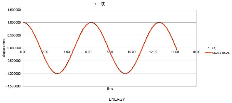
In order to study the thermodynamic properties of a system we generate a system made up of N atoms, each of them obeying Newton’s second law. Since in this way a very large number of equations would be generated, the velocity - Verlet algorithm is used to tackle the data. The results obtained by the application of this algorithm show good agreement with the classical solutions of the same problem. This is shown below in the example of the classic oscillator. Arbitrary values are provided for the constants.

The red line represents the position as calculated classically via the relationship:

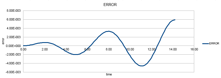
The blue dots are the values of the position generated via the velocity - Verlet algorithm for a timestep value of 0.1. The difference between the classical and velocity - Verlet values is plotted against time:

The error in the value of the position changes with time in this way because the velocity - Verlet algorithm ignores all terms of the Taylor expansion except the first two and therefore has an error of the order of Δt₂ at long times.

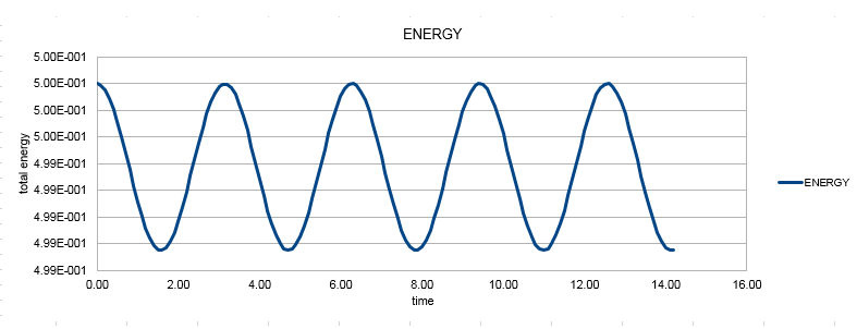
Monitoring the total energy is important to ensure that the simulation generated reflects reality and therefore the results obtained are reliable. Total energy must remain constant since the system obeys to the law of the conservation of energy. If the variation in the value of the energy is too large then the parameters of the simulation will have to be changed. The total energy of the oscillator is then plotted based on the values of velocity and displacement obtained by the velocity - Verlet algorithm.

The value of the energy shows a slight variation over time, by 0.25% for this value of the timestep. To ensure that the total energy does not change by more than 1%, the timestep used in the calculation must be lower than 0.2.

Interatomic interactions

The pairwise interactions between the atoms of the system are modelled by the Lennard – Jones potential. For a single interaction:

The separation r₀, at which the potential energy is equal to zero, is therefore equal to σ. The separation at equilibrium, r_eq can be found by setting the differential of the potential energy equal to zero, since at equilibrium the system has its minimum potential energy.

In this way it is found that and where φ(r_eq) is the well depth of the potential curve.

The following integrals are calculated (σ = є = 0.1):

For 2.5σ and 3.0σ the values obtained by the integrals are quite small which supports the decision of excluding them from the results.

Periodic boundary conditions

The simulation that is produced should provide results close to experimental values for a bulk fluid, regarding quantities such as density, diffusion coefficient etc. However the number of molecules found in a bulk liquid is very large while the number of molecules that can be simulated is limited. Considering for example the number of water molecules that make up 1mL of water under standard conditions it would be as calculated below:

In the simulation however the number of molecules is set between 1000 and 10000 molecules. The volume of 10000 water molecules under standard conditions is found as shown below:

To overcome this limitation a simulation box is generated in which the atoms are enclosed. This box is repeated on all directions infinite times so that the end result resembles a bulk liquid.

Boundary conditions are in effect according to which the moving atoms can leave the box only to enter it again on the other side since they enter a replica of the initial cell.

For example an atom is initially at the centre of a cubic simulation box which runs from (0, 0, 0) to (1, 1, 1). If this atom moves along the vector (0.7, 0.6, 0.2) there are several possibilities about its position after a single timestep.

1. The atom didn't leave the box. Its new position is then (0.5+0.7t, 0.5+0.6t, 0.5+0.2t). 2. The atom left the box. This occurs if its position in the x, y or z axis becomes larger than 1. In this case each dimension has to be considered separately.

If the x value becomes larger than 1 then with the new boundary conditions the atom's position on the x axis will become 0.5 + 0.7t - 1. If the y value becomes larger it will be changed to 0.5 + 0.6t - 1 and if the z value becomes larger than 1 then the new position on the z axis will be 0.5 + 0.2t - 1.

Since by applying the boundary conditions it can be now assumed that we have a bulk solution, a distance limit has to be placed on the interactions between the atoms, otherwise the total energy of the system will be infinite. Therefore a limit is defined above which interactions can be ignored. This is usually set at 2.5σ or 3.0σ.

Another thing to keep in mind is that all the quantities used in the simulation are given in reduced units. The conversion is given below for the values of distance, energy and temperature:

So for example, given that in the case of argon σ = 0.34 nm and є/k_B = 120 K, then the Lennard - Jones cutoff value, r* = 3.2, is in fact equal to:

The well depth є is equal to:

Finally, T* = 1.5 is equal to:

Equilibration

The aim of this part of the exercise was to determine the ideal timestep for the calculations by considering the difference in the time it took for a system to reach equilibrium when varying the timestep value. For this purpose simple simulations were run with a different timestep value each time so that the results could be compared.

Input file analysis

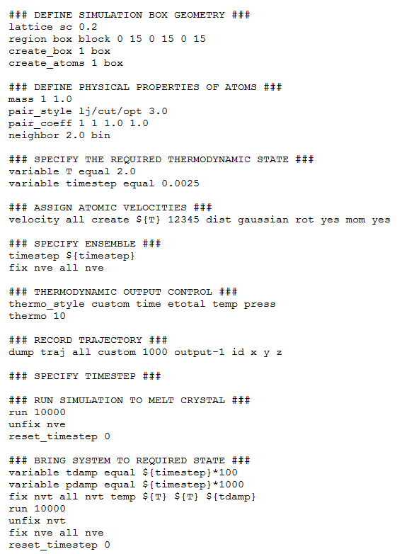
The structure of a liquid is disordered which poses a problem when defining the initial position of the atoms. Generating random positions for the atoms would be a bad idea because it could lead to overlap of the atoms and unfavourable interactions. To overcome this problem a crystal lattice is generated and then melted to form the liquid.

The commands given to the program asked for the creation of a simple cubic lattice with 0.8 lattice points per cell. The program therefore generated a simple cubic lattice with lattice points at a distance of 1.07722 from each other. This indeed corresponds to the lattice specified as shown:

Since the lattice is simple cubic each of the sides of the unit cell is equal to 1.07722 and the volume is equal to:

Each unit cell contains 1 lattice point (simple cubic) therefore the number density (number of lattice points per unit volume) is equal to:

If instead of this lattice we had a face centred cubic lattice, which contains 4 lattice points per unit cell, of density 1.2, then the side length of the unit cell would be:

Next, a command was given to form a lattice containing 10 x 10 x 10 = 1000 unit cells. Since the lattice type was simple cubic this meant that 1000 atoms were generated. If the lattice was face centred cubic the total amount of atoms would be 4000.

By looking through the rest of the input file the following commands were found. The role of each command is given:

mass 1 1.0: defines the value of the mass of type 1 atoms (in this case all the atoms since there is only one type) to be 1.0

pair_style lj/cut 3.0: states that pair-wise interactions are to be considered negligible at a distance of 3.0σ and above

pair_coeff * * 1.0 1.0: defines the values of the pairwise force field constants I and J as 1.0 and 1.0

Since in the input file both x_i(0) and v_i(0) are specified the integration logarithm used for the calculations is the velocity – Verlet algorithm.

The following command was given for the execution of the calculation:

The timestep was defined as a variable so that its value could be easily modified in later calculations by simply changing the line in the input script that defines the timestep:

Variable timestep equal …

The time over which the simulation takes place is defined in such a way in order to have 100 timesteps in total. So even if the value of the timestep changes the number of timesteps doesn't.

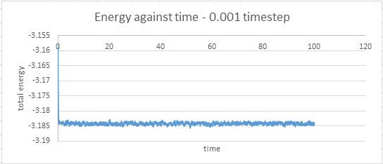
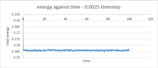
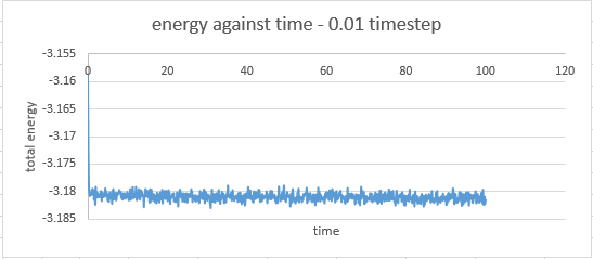
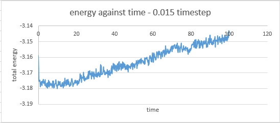
The total energy of the system was subsequently calculated by the program and it was plotted against time in order to determine the time it took for the system to reach equilibrium in each case.

Results analysis

The times at which each system reached equilibrium were:

timestep 0.001: at 0.42

timestep 0.0025: at 0.43

timestep 0.0075: at 0.45

timestep 0.01: at 0.5

timestep 0.015: the system didn't reach equilibrium

A very small timestep may be precise but it leads to very time consuming calculations. On the other hand a large time step leads to mistakes in the integration of the equations of motion or to very large energy changes and eventually destabilizes the integrating algorithm. This particularly obvious in the case where the 0.015 timestep was used as the system never reached equilibrium.

The timestep chosen for subsequent calculations was 0.0025 because it was the largest to give acceptable results. The value of energy obtained by this particular calculation showed less fluctuation than in the cases where the 0.0075 and 0.001 timesteps were used. The average value of energy was also larger in magnitude than those obtained from the 0.0075 and 0.01 timestep simulations, but similar to that obtained by the 0.001 timestep simulation.

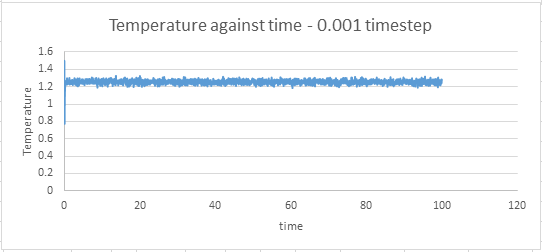
The values of temperature and pressure were plotted against time for the 0.001 timestep simulation.

Running simulations in the isobaric - isothermal ensemble

In this part of the exercise the simulations used in the previous section were modified so that they could be run in the NpT (isobaric - isothermal) ensemble. Temperature and pressure were therefore specified as variables. The simulation was then run at two different values of pressure (2.5 and 3.5) and five different values of temperature (2.0, 5.0, 10.0, 20.0 and 50.0) so that ten runs were obtained in total.

The reduced pressure is given by .

Temperature control

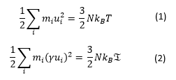
Using the equipartition principle the following relationships are generated:

where T is the instantaneous temperature of the system while is the temperature which we aim to reach and which is specified in the input file.

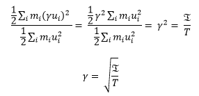
Equation (2) is divided by equation (1):

Therefore to reach the desired temperature, , γ must become equal to 1.

Input file analysis

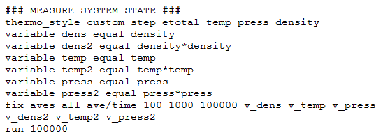
The input file contains the lines:

The three numbers 100 1000 100000 in the command “fix aves all ave/time 100 1000 100000 v_dens v_temp v_press v_dens2 v_temp2 v_press2” mean:

use the input values every 100 timesteps

use the input values for calculating the averages 1000 times

calculate the averages every 100000 timesteps

The values of the variables will be sampled for the average every 100 timesteps. 1000 measurements contribute to the calculation of the averages. The equivalent of 100000 timesteps (100000 x 0.0025 = 250) will be simulated.

Plotting the equations of state

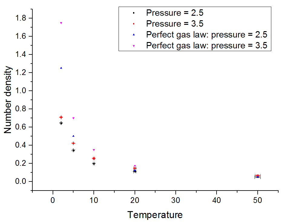
Density was plotted against temperature for both values of the pressure. The errors in the values of density and temperature are included. In the same graph were plotted the values of density predicted by the ideal gas law for the given temperatures.

From the graph it can be deduced that the density predicted by the ideal gas law is higher than that generated by the simulation. This of course is expected to be the case because the ideal gas law ignores any intermolecular interactions. This discrepancy increases with increasing pressure, because the increase leads to more frequent intermolecular interactions.

Calculating heat capacities

Heat capacity can be calculated in statistical thermodynamics by the following relationship:

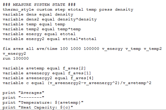
The input file used in the previous section was modified in order to calculate the heat capacity as shown:

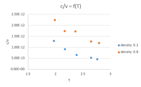
This simulation was run for two different values of density and five values of temperature (ten runs in total). The values of heat capacity obtained were divided by the volume of the simulation box at the specified density (V = 16874.92263 for a density of 0.2 and V = 4218.781194 for a density of 0.8) and then they were plotted against temperature.

The value of heat capacity decreases as the temperature increases. This is not what we would expect. The relationship between heat capacity and temperature which is: , where a,b and c are constants and a,b are positive while c is negative. For large values of T the positive term should prevail.

As density increases heat capacity increases. This also is not as expected as generally heat capacity decreases as density increases.

Structural properties and the radial distribution function

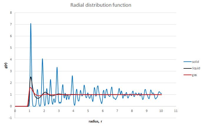
In this part of the exercise the radial distribution functions of the system in the solid, liquid and gaseous phases were plotted. The radial distribution function shows the average positions of the atoms relative to each other and its examination provides information about the structural properties of the system.

Three simulations were run for the same system, one in each state. The state of the system was controlled in each case by varying the temperature and the lattice density. In order to determine the appropriate conditions for each simulation the phase diagram of the Lennard - Jones system was examined. The conditions imposed were:

for the solid state: density = 1.1, temperature = 0.3, lattice type: face-centred cubic

for the liquid state: density = 0.8, temperature = 1.2

for the gaseous state: density = 0.55, temperature = 4.5

The radial distribution functions obtained are shown below:

A face of the FCC unit cell showing the peak assignments

The radial distribution function of the system in the solid state is a series of sharp peaks, showing that the atoms lie at specific positions in the lattice and therefore at specific distances from a reference atom. The peaks are still discrete even at large distances so the system is said to have long-range order [R]. This long-range order is lost in the liquid and gaseous phases as the atoms are free to move in space meaning that the probability of finding another atom is the same everywhere. However a short-rage order is still retained as the atoms nearest to the reference atom might adopt positions similar to those they had in the solid state. This is mainly observed in the case of the liquid simulation. In the gaseous phase there is considerably less order.

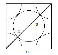
The first three peaks of the solid state radial distribution plot can be assigned since the lattice type is known as shown to the left.

r1 corresponds to the first peak, r2 to the second and r3 to the third.

The lattice spacing is equal to 1.435.

As the lattice type is face centred planar the coordination number is 12.

Dynamical properties and the diffusion coefficient

The diffusion coefficient of the systems can be calculated based on the following relationship:

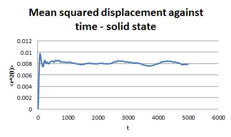
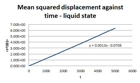
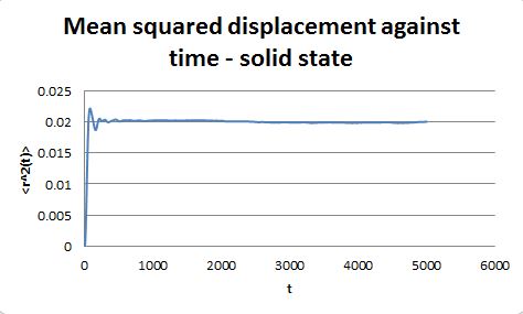
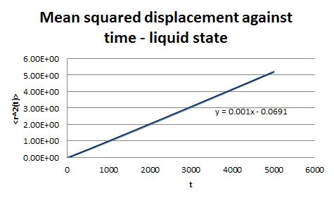
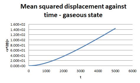
For the simulations generated in the previous part, the mean square displacement was measured and plotted against time for the solid, liquid and gas phases.

The shape of these plots is roughly as expected. The plot corresponding to the solid shows that the atoms are not free to move in space and can only vibrate around fixed positions. In the case of the liquid and the gas the atoms can move freely and therefore their displacement changes with time.

From the gradient of these plots the diffusion coefficient D can be determined.

gradient = 6D

Therefore for the liquid phase D = 2.14 x 10^-4 and for the gaseous phase D = 1.73 x 10^-3.

All these values of D have to me multiplied by the appropriate conversion factor in order to obtain the correct units. The dimensions of D are distance² over time.

The same procedure was repeated for simulations containing one million atoms.

gradient = 1.05 x 10^-3, therefore D = 1.75 x 10^-4

gradient of the linear part = 3.62 x 10^-2, therefore D = 6.03 x 10^-3

Velocity autocorrelation function

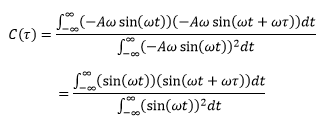
The velocity autocorrelation function of the harmonic oscillator can be obtained by substituting the classical velocity relationship the equation given below as shown:

The relationship obtained will be a periodic function.

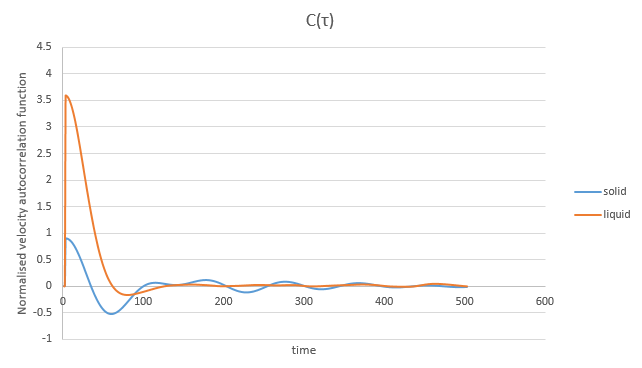
Shown below on the same graph are the velocity autocorrelation function against time plots obtained for the solid and liquid simulations previously performed.

In the case of the solid some oscillation is observed at large times due to the fact that the atoms vibrate at fixed positions, while in the case of the liquid this does not take place.

The graph that would be obtained in the case of the harmonic oscillator would be very different to the graphs of both the solid and the liquid because its oscillation is preserved over time.