CMP Monte Carlo Simulation - Alwin Bucher

The Ising Model

The Ising model is one of the simplest physical models to display a phase transition, consisting only of spins interacting with their nearest neighbours, and yields insight into the behaviour of a variety of physical systems, such as gases and ferromagnetic materials.

Assuming that the Ising lattice adopts an equally spaced chain in one, a square lattice in two, a cubic lattice in three dimensions, and the analogous structures in higher dimensions, it becomes clear that each lattice site in the bulk has $2 D$ nearest neighbours, where $D$ is the number of dimensions. Periodic boundary conditions are implemented in order to simulate large-scale systems, and thus the spins located on the edges of the simulation box interact with the spin directly opposite, as if the simulation box was tied to itself in a ring. All spins therefore interact with $2 D$ nearest neighbours.

Energy and Entropy

In the absence of an external magnetic field, the energy of an Ising lattice is given by $E = - \frac{1}{2} J \sum_{i} \sum_{j \in n e i g h b o u r s (i)} s_{i} s_{j}$ . If the spin of lattice site $i$ takes values of either $+ 1$ or $- 1$ , the lattice energy is at a minimum when all spins are the identical. Thus, $E_{m i n} = - \frac{1}{2} J \sum_{i} \sum_{j \in n e i g h b o u r s (i)} s^{2} = - \frac{1}{2} J \sum_{i} \sum_{j \in n e i g h b o u r s (i)} 1$ .

The energy thus further reduces to $E = - \frac{1}{2} J \sum_{i} 2 D = - J N D$ , where $N$ is the number of spins in the lattice, and $J$ a parameter representing the absolute interaction energy of two adjacent spins, which, in reduced units (which are used throughout this report when numerical quantities are computed), is equal to $k_{B}$ .

As mentioned, this state is obtained when either all spins are $+ 1$ or $- 1$ , and thus its multiplicity is 2. Since entropy is related to the multiplicity $Ω$ by $S = k_{B} \ln (Ω)$ , the entropy of this state is $k_{B} \ln (2) = 9.57 \times 1 0^{- 24} J / K$ .

Alternatively, the configurations with all spins $+ 1$ or $- 1$ may be considered as two separate states (if magnetisation states rather than energy states are of interest), in which case the entropy of both is zero, since $\ln (1) = 0$ .

Phase Transitions

Any transition from a system initially in the state of minimum energy described in the previous section must go through a state where all but one spin are either $+ 1$ or $- 1$ . Since periodic boundary conditions have been imposed, all lattice sites are equivalent, and so the multiplicity of this state is $2 N$ , where the factor of $2$ accounts for the fact that the spin of all but one of the spins can be either $+ 1$ or $- 1$ . The corresponding entropy change for $N = 1000$ is therefore $Δ S = k_{B} \ln (2 N) - k_{B} \ln (2) = k_{B} \ln (N) = 3 k_{B} \ln (10) = + 9.54 \times 1 0^{- 23} J / K$ .

The change in energy of the Ising lattice as a consequence on the above transition is simply the change in energy of the interaction between the flipped spin and its nearest neighbours, since the rest of the lattice does not 'feel' the change. As it is a 3-dimensional lattice that is being considered, there are 6 of these interactions, and thus the energy change is $+ 12 J$ .

Magnetisation

The magnetisation $M$ of an Ising lattice is simply given by $M = \sum_{i} s_{i}$ , i.e. the sum of all the spins. Thus, the magnetization of the 1- and 2-dimensional lattices given in figure 1 in the task wiki page is 1.

At $0 K$ , there is no thermal energy available to excite the lattice into any higher-energy states by flipping a single spin, and thus the Ising lattice is certain to occupy the state of minimum energy previously described. Thus, the magnetisation of a three-dimensional $10 \times 10 \times 10$ Ising lattice will be $\pm 1000$ .

Writing a Monte-Carlo Simulation

Testing the Energy and Magnetisation Code

Below is the code of the energy() and magnetisation() functions, prior to acceleration of the code.

    def energy(self):
        "Return the total energy of the current lattice configuration."
        energy = 0
        lat = self.lattice
        x = self.n_rows - 1
        y = self.n_cols - 1
        
        #Compute energy contributions from corner sites
        energy += -1/2 * lat[0][0]*(lat[1][0] + lat[x][0] + lat[0][1] + lat[0][y]) 
        energy += -1/2 * lat[x][0]*(lat[x][1] + lat[x][y] + lat[x-1][0] + lat[0][0])
        energy += -1/2 * lat[x][y]*(lat[x-1][y] + lat[0][y] + lat[x][y-1] + lat[x][0])
        energy += -1/2 * lat[0][y]*(lat[1][y] + lat[x][y] + lat[0][y-1]+ lat[0][0])
        
        #Compute energy contributions from edge and bulk sites
        i = 1
        while i < x:
            energy += -1/2 * lat[i][0]*(lat[i][1] + lat[i][y] + lat[i-1][0] + lat[i+1][0])
            energy += -1/2 * lat[i][y]*(lat[i][y-1] + lat[i][0] + lat[i-1][y] + lat[i+1][y])
            j = 1
            while j < y:
                energy += -1/(2*(x-1)) * lat[0][j]*(lat[1][j] + lat[x][j] + lat[0][j-1] + lat[0][j+1])
                energy += -1/(2*(x-1)) * lat[x][j]*(lat[x-1][j] + lat[0][j] + lat[x][j-1] + lat[x][j+1])
                energy += -1/2 * lat[i][j]*(lat[i][j+1] + lat[i][j-1] + lat[i+1][j] + lat[i-1][j])
                j += 1
            i += 1
        return energy

    def magnetisation(self):
        "Return the total magnetisation of the current lattice configuration."
        magnetisation = 0.0
        for i in self.lattice:
            for j in i:
                magnetisation += j
        return magnetisation

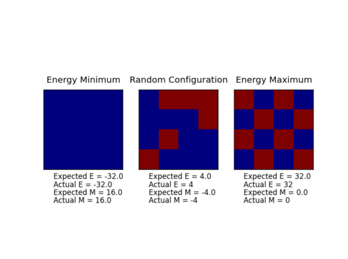
The output of ILcheck.py is shown in figure 1.

Average Energy and Magnetisation

A system of 100 spins can access $2^{100} \approx 1.3 \times 1 0^{30}$ spin configurations. Assuming that per second, the energy and magnetisation of $1 \times 1 0^{9}$ configurations can be computed, the time required would be $1.3 \times 1 0^{21} s \equiv 1.6 \times 1 0^{16} d a y s$ , clearly an unreasonable amount of time!

A much more sensible approach is to calculate the average energy and magnetisation only over a much smaller sample of states, whose distribution matches that of all states. A commonly used algorithm which accomplishes this quite effectively forms the basis of the Metropolis Monte Carlo method. ^[1]

The code of the montecarlostep() and statistics() functions, prior to choosing an initial number of steps over which no data is collected, is shown below:

    def montecarlostep(self, T):
        # These lines add the current values to the cumulative totals
        oldEnergy = self.energy().copy()
        oldMag = self.magnetisation().copy()
        self.E += oldEnergy
        self.M += oldMag
        self.E2 += oldEnergy**2
        self.M2 += oldMag**2
        
        #the following two lines will select the coordinates of the random spin for you
        random_i = np.random.choice(range(0, self.n_rows))
        random_j = np.random.choice(range(0, self.n_cols))
        # Copies the previous lattice in case the change is not accepted
        oldLattice = self.lattice.copy()
        # Randomly flips a spin of the current lattice
        newLattice = self.lattice
        newLattice[random_i][random_j] = -1 * oldLattice[random_i][random_j]
        self.lattice = newLattice
        # Computes change in energy 
        newEnergy = self.energy()
        deltaE = newEnergy - oldEnergy
        # Either accepts or rejects new lattice
        if deltaE > 0:
            random_number = np.random.random()
            if random_number > np.exp(-deltaE/T):
                self.lattice = oldLattice
        magnetisation = self.magnetisation()
        energy = self.energy()
        self.n_cycles += 1
        return [energy,magnetisation]

    def statistics(self):
        AveE = self.E/(self.n_cycles)      
        AveE2 = self.E2/(self.n_cycles)
        AveM = self.M/(self.n_cycles)      
        AveM2 = self.M2/(self.n_cycles)
        return [AveE,AveE2,AveM,AveM2]

At temperatures below the critical (or Curie) temperature, the energetically favourable interactions dominate over the entropic driving fource, and thus spontaneous magnetisation is expected to occur. This is borne out by the output of ILanim.py, shown in figure 2.

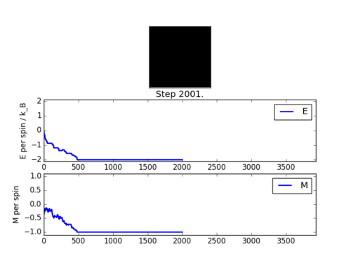
The values of $⟨ E ⟩$ , $⟨ E^{2} ⟩$ , $⟨ M ⟩$ and $⟨ M^{2} ⟩$ as computed by the statistics() function are -116.5, 14140, -56.77 and 3445 respectively. Note that the energies and magnetisations plotted in figure 2 are per spin, and so a factor of 64 is necessary for comparison between these and the values output by the statistics() function. Clearly, the final lattice energy of -120 is somewhat more negative than the average energy of -116.5, as a result of the average energy being computed over all of the simulation, including the steps prior to convergence.

Accelerating the Code

Computing the energy and magnetisation by iterating over all lattice elements using nested loops is very computationally inefficient. Alternatively, the use of pre-written functions which sum all elements of a matrix (np.sum()), shift all elements of a matrix along a given axis by a given number of indices (np.roll()) and multiply matrices elementwise (np.multiply()) significantly speed up the simulation. The code of the modified functions is given below.

    def energy(self):
        "Return the total energy of the current lattice configuration."
        energy = -1*np.sum(np.multiply(self.lattice,np.roll(self.lattice,1,0)))
        energy += -1*np.sum(np.multiply(self.lattice,np.roll(self.lattice,1,1)))
        return energy

    def magnetisation(self):
        "Return the total magnetisation of the current lattice configuration"
        return np.sum(self.lattice)

It should be noted that np.roll() re-introduces elements which shift beyond the last position at the first position, which corresponds to implementing periodic boundary conditions. The times taken to complete 2000 steps of the Monte-Carlo simulation using nested loops and the mentioned functions are $37 \pm 1 s$ and $0.27 \pm 0.01 s$ respectively. These values represent the means and standard deviations over 25 repeat measurements. The ILtimetrial.py script was modified in the following way to allow for automation of repeat measurements:

import time
import IsingLattice as il
import numpy as np

#use a relatively big lattice of 25x25 so that we get more accurate timing data
n_rows = 25
n_cols = 25
elapsed_times = []
for i in range(0,25):
    lattice = il.IsingLattice(n_rows, n_cols)
    #record the time at which we start running
    start_time = time.clock()
    #do 2000 monte carlo steps
    for i in range(2000):
        lattice.montecarlostep(1.0)
    #record the time at which we stop running
    end_time = time.clock()
    
    #work out how many seconds the loop took, and print it
    elapsed_time = end_time - start_time
    elapsed_times.append(elapsed_time)
    
std = np.std(elapsed_times)
mean = np.mean(elapsed_times)
print(std,mean)

Adjusting the Average

To compute an average value of the converged energy and magnetisation of a simulation, the statistics() and montecarlostep() functions adjusted such as to only average the energies after an initial $N$ cycles:

    def montecarlostep(self, T):
        # These lines add to the cumulative totals after an initial 1000 steps
        oldEnergy = self.energy()
        oldMag = self.magnetisation()
        if self.n_cycles > 1000:
            self.E += oldEnergy
            self.M += oldMag
            self.E2 += oldEnergy**2
            self.M2 += oldMag**2
            self.aM += abs(oldMag)
        #the following two lines will select the coordinates of the random spin for you
        random_i = np.random.choice(range(0, self.n_rows))
        random_j = np.random.choice(range(0, self.n_cols))
        # Copies the previous lattice in case the change is not accepted
        oldLattice = self.lattice.copy()
        # Randomly flips a spin of the current lattice
        newLattice = self.lattice
        newLattice[random_i][random_j] = -1 * oldLattice[random_i][random_j]
        self.lattice = newLattice
        # Computes change in energy 
        newEnergy = self.energy()
        deltaE = newEnergy - oldEnergy
        # Either accepts or rejects new lattice
        if deltaE > 0:
            random_number = np.random.random()
            if random_number > np.exp(-deltaE/T):
                self.lattice = oldLattice
        magnetisation = self.magnetisation()
        energy = self.energy()
        self.n_cycles += 1
        return [energy,magnetisation]
        
    def statistics(self):
        AveE = self.E/(self.n_cycles -1000)
        AveE2 = self.E2/(self.n_cycles-1000)
        AveM = self.M/(self.n_cycles -1000)
        AveM2 = self.M2/(self.n_cycles -1000)
        AveaM = self.aM/(self.n_cycles -1000)
        return [AveE,AveE2,AveM,AveM2,self.n_cycles,AveaM]

The number $N$ was chosen in the following way:

the speed of convergence of a Monte-Carlo simulation was found to vary with temperature and lattice size. In particular, it increased with lattice size, as can be seen by comparing figures 3 and 4.

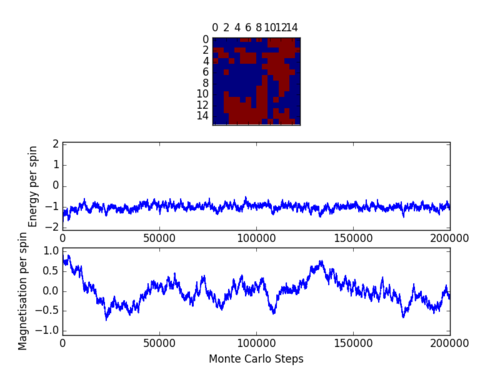
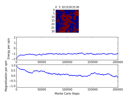
A point of interest in the above figures are the comparatively larger fluctuations in the magnetisation per spin of the $16 \times 16$ (figure 3) than of the $32 \times 32$ lattice (figure 4). This is simply a result of the smaller number of spins in the $16 \times 16$ lattice - the effect of the inversion of a single spin on the total magnetisation is far more significant.

However, the above plots are not an accurate measure of the speed of convergence of the simulation in the context of the ILtemperaturerange.py script provided, as the Ising lattice at each temperature step is initialised with the converged lattice at the previous temperature, and with the all $+ 1$ configuration for each first temperature step. If reasonably small temperature spacing are used, the average structure of the Ising lattices at adjacent data points will be likely to be much more similar than the initial random lattice and the final converged lattices - which fluctuate about $⟨ M ⟩ = 0$ - shown in figures 3 and 4. Thus, only approximately 1000 steps are required to convergence and prior to inclusion of the energies and magnetisations in the final statistical quantities, which were collected over a range of 198000 steps, in agreement with results obtained by J. Kotze ^[2]. The resulting graphs are shown in figures 5 to 10.

Temperature and Lattice Size Dependence of Energy and Magnetisation

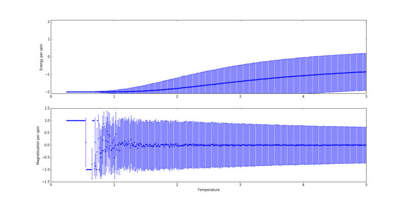
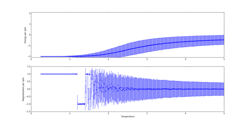
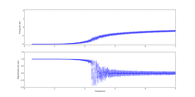
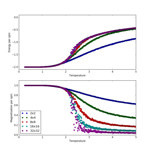
Figures 5 to 9 were chosen to be plotted separately as the overlap between errorbars was found to detrimentally affect their clarity. To illustrate the dependency on lattice size, a collective plot with the omission of error bars is shown in figure 10.

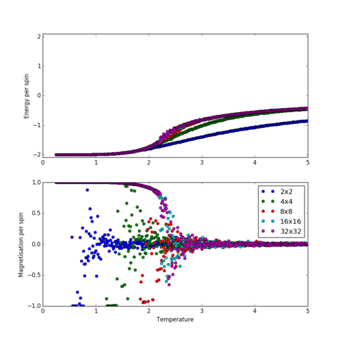
From these figures, it can be seen that the temperature at which the average magnetisation drops close to zero increases with lattice size.

This effect can be explained by the fact that, due to the finite size of the Ising lattices, there is a finite probability that a lattice with, for example, initially all spins $+ 1$ can completely flip to a configuration where all spins are in the $- 1$ state. The probability of this occurring increases with temperature and inversely with lattice size, since the number of high-energy configurations which have to be traversed increases with lattice size, and the probability of each unfavourable spin inversion required in the process increases with temperature. Since all configurations with the same energy are equally likely, as $t \to \infty$ we expect $⟨ M ⟩ \to 0$ if there is even a finite probability of the described inversion of the lattice. Clearly, only at $T = 0$ is this probability zero, but of course only finite simulations can be performed. Thus, at low temperatures, no such lattice flipping is seen. Upon increasing the temperature, a random distribution of $⟨ M ⟩$ between $+ 1$ and $- 1$ is observed (at temperatures where the total probability of a flip over a 200000 step simulation is on the order of 1 and thus the magnetisation is not significantly more likely to average out to 0 than any other number between -1 and +1), followed by $⟨ M ⟩ = 0$ at temperatures where such flips occur with such frequency that for time spend in every state with magnetisation +M, a roughly equal amount of time is spent in a state with magnetisation -M.

Clearly then, the decay to zero of the average magnetisation of smaller lattices at lower temperatures is not a result of a disordered state, as would be expected above the Curie temperature, but of rapid switching between highly magnetised states of opposite magnetisations. This corroborates the trends of the energy with lattice size and temperature seen in figure 10, as states with larger absolute magnetisation are, on average, lower in energy than those with low magnetisation. To see this more clearly, a plot of the average absolute magnetisation analogous to figure 10 is shown in figure 11. As can be seen, the average absolute magnetisation in fact decays less rapidly with temperature for smaller lattices. This, and the similar trend in energy, can be explained by the dependency of the ratio of the multiplicities of disordered and ordered states with lattice size. Clearly, the multiplicity of the most disordered state increases rapidly with lattice size, whilst that of the lowest energy state with $M \pm N$ remains constant at 2. As a result, the entropic driving force favours the disordered state much more strongly at larger lattice sizes, producing the observed steepening of the gradient of $⟨ E ⟩$ and $⟨ | M | ⟩$ past a certain temperature - the Curie temperature.

The described long-range fluctuations are of course an entirely physical phenomenon - they simply do not occur from the low-energy configurations where nearly all spins are aligned in a macroscopic lattice, since the number of unfavourable inversions of individual spins required would be astronomical. In a periodic $2 \times 2$ lattice however, only two of such are required for the lattice to reach the highest-energy conformation, following which it is equally likely to either return to the original state, or collapse into the other state where all spins are aligned. Thus, this transition takes place at far lower temperatures than should be possible. Of course, at greater temperatures the entropic driving force will play a more significant role, and thus the equilibrium configuration will be more disordered, have higher energy and as a result require fewer unfavourable spin flips to reach a configuration with equal energy but opposite magnetisation.

From the preceding analysis, it can be concluded that a simulated Ising lattice using periodic boundary conditions accurately represents the behaviour of a macroscopically large Ising lattice only if complete inversions in the magnetisation of the lattice only occur near the Curie temperature, in other words, when the equilibrium configuration of the lattice is significantly disordered.

Looking at figures 5 - 10, it becomes apparent that this criterion is only somewhat satisfied for a $16 \times 16$ lattice. Clearly, the 'correctness' of these fluctuations increases monotonously with the lattice size. However, the rate of increase in 'correctness' with lattice size rapidly diminishes, as can be seen in figure 11, where the curves corresponding to the $16 \times 16$ and $32 \times 32$ lattices are virtually superimposed. Thus, to answer the question "How big a lattice do you think is big enough to capture the long range fluctuations?", I would say that the answer is a matter of the required accuracy of the results deriving from the variance in energy and magnetisation, such as the heat capacity and magnetic susceptibility of the lattice, but certainly no less than a $16 \times 16$ lattice.

Figures 5 - 9 were created using:

import pylab as pl
import numpy as np
for i in [2,4,8,16,32]:
    print(i)
    temps,energies,energysq,magnetisations,magnetisationsq,aMs = np.loadtxt(str(i) + '_full_200000_with_abs.dat',unpack=True)
    Std_E = (np.array(energysq)-np.array(energies)**2)**0.5/i**2
    Std_M = (np.array(magnetisationsq)-np.array(magnetisations)**2)**0.5/i**2
    fig = pl.figure(figsize=(20,10))
    enerax = fig.add_subplot(2,1,1)
    enerax.set_ylabel("Energy per spin")
    magax = fig.add_subplot(2,1,2)
    magax.set_ylabel("Absolute magnetisation per spin")
    magax.set_xlabel("Temperature")
    enerax.errorbar(temps,np.array(energies)/i**2,yerr=Std_E,fmt='.')
    magax.errorbar(temps,np.array(magnetisations)/i**2,yerr=Std_M,fmt='.')
    pl.show()

Figure 10 was created using:

import pylab as pl
import numpy as np
Es = []
Mgs = []
for i in [2,4,8,16,32]:
    print(i)
    temps,energies,energysq,magnetisations,magnetisationsq,aMs = np.loadtxt(str(i) + '_full_200000_with_abs.dat',unpack=True)
    Es.append(energies/i**2)
    Mgs.append(magnetisations/i**2)
fig = pl.figure(figsize=(10,10))
enerax = fig.add_subplot(2,1,1)
enerax.set_ylabel(r'$\langle E \rangle$')
enerax.set_xlabel("Temperature")
enerax.set_ylim([-2.1, 0.1])
magax = fig.add_subplot(2,1,2)
magax.set_ylabel(r'$\langle M \rangle$')
magax.set_xlabel("Temperature")
magax.set_ylim([-1.1, 1.1])
enerax.plot(temps,np.array(Es[0]),linestyle='none',marker='o',label='2x2')
enerax.plot(temps,np.array(Es[1]),linestyle='none',marker='o',label='4x4')
enerax.plot(temps,np.array(Es[2]),linestyle='none',marker='o',label='8x8')
enerax.plot(temps,np.array(Es[3]),linestyle='none',marker='o',label='16x16')
enerax.plot(temps,np.array(Es[4]),linestyle='none',marker='o',label='32x32')
magax.plot(temps,np.array(Mgs[0]),linestyle='none',marker='o',label='2x2')
magax.plot(temps,np.array(Mgs[1]),linestyle='none',marker='o',label='4x4')
magax.plot(temps,np.array(Mgs[2]),linestyle='none',marker='o',label='8x8')
magax.plot(temps,np.array(Mgs[3]),linestyle='none',marker='o',label='16x16')
magax.plot(temps,np.array(Mgs[4]),linestyle='none',marker='o',label='32x32')
pl.legend(loc='best')
pl.show()

And figure 11 using:

import pylab as pl
import numpy as np
Es = []
aMgs = []
for i in [2,4,8,16,32]:
    print(i)
    temps,energies,energysq,magnetisations,magnetisationsq,aMs = np.loadtxt(str(i) + '_full_200000_with_abs.dat',unpack=True)
    Es.append(energies/i**2)
    aMgs.append(aMs/i**2)
fig = pl.figure(figsize=(10,10))
enerax = fig.add_subplot(2,1,1)
enerax.set_ylabel(r'$\langle E \rangle $')
enerax.set_xlabel("Temperature")
enerax.set_ylim([-2.1, 0.1])
magax = fig.add_subplot(2,1,2)
magax.set_ylabel(r'$\langle |M| \rangle$')
magax.set_xlabel("Temperature")
magax.set_ylim([0, 1.1])
enerax.plot(temps,np.array(Es[0]),linestyle='none',marker='o',label='2x2')
enerax.plot(temps,np.array(Es[1]),linestyle='none',marker='o',label='4x4')
enerax.plot(temps,np.array(Es[2]),linestyle='none',marker='o',label='8x8')
enerax.plot(temps,np.array(Es[3]),linestyle='none',marker='o',label='16x16')
enerax.plot(temps,np.array(Es[4]),linestyle='none',marker='o',label='32x32')
magax.plot(temps,np.array(aMgs[0]),linestyle='none',marker='o',label='2x2')
magax.plot(temps,np.array(aMgs[1]),linestyle='none',marker='o',label='4x4')
magax.plot(temps,np.array(aMgs[2]),linestyle='none',marker='o',label='8x8')
magax.plot(temps,np.array(aMgs[3]),linestyle='none',marker='o',label='16x16')
magax.plot(temps,np.array(aMgs[4]),linestyle='none',marker='o',label='32x32')
pl.legend(loc='best')
pl.show()

The data used was generated using a modified version of ILtemperaturerange.py:

from IsingLattice import *
from matplotlib import pylab as pl
from matplotlib import pyplot as plt
import numpy as np
for n_rows in [2,4,8,16,32]:
    print(n_rows)
    n_cols = n_rows
    il = IsingLattice(n_rows, n_cols)
    il.lattice = np.ones((n_rows, n_cols))
    spins = n_rows*n_cols
    runtime = 1002000
    times = range(runtime)
    temps = np.arange(0.25, 5.0, 0.01)
    energies = []
    magnetisations = []
    energysq = []
    magnetisationsq = []
    absMag = []
    for t in temps:
        for i in times:
            energy, magnetisation = il.montecarlostep(t)
        aveE, aveE2, aveM, aveM2, n_cycles, AveaM = il.statistics()
        energies.append(aveE)
        energysq.append(aveE2)
        magnetisations.append(aveM)
        magnetisationsq.append(aveM2)
        absMag.append(AveaM)
        #reset the IL object for the next cycle
        il.E = 0.0
        il.E2 = 0.0
        il.M = 0.0
        il.M2 = 0.0
        il.n_cycles = 0
        il.aM = 0.0
    Std_E = (np.array(energysq)-np.array(energies)**2)**0.5/spins
    Std_M = (np.array(magnetisationsq)-np.array(magnetisations)**2)**0.5/spins
    final_data = np.column_stack((temps, energies, energysq, magnetisations, magnetisationsq,absMag))
    np.savetxt(str(n_cols) + "_full_1000000_with_abs.dat", final_data)

Calculating the Heat Capacity

The constant-volume heat capacity of a system is given by $C_{v} = \frac{\partial ⟨ E ⟩}{\partial T}$ . The expectation value of the energy of a two-dimensional Ising lattice is in turn $⟨ E ⟩ = \frac{1}{Z} \sum_{α} E (α) e^{- \frac{E (α)}{k_{B} T}}$ where $α$ is an index over all states and $Z = \sum_{α} e^{- \frac{E (α)}{k_{B} T}}$ the partition function ^[3]. In the following, $β = \frac{1}{k_{B} T}$ .

$C_{v} = \frac{\partial ⟨ E ⟩}{\partial T} = \frac{\partial β}{\partial T} \frac{\partial ⟨ E ⟩}{\partial β}$ .

Substituting for $β$ , we can write:

$Z = \sum_{α} e^{- β E (α)} ⟹ \frac{\partial Z}{\partial β} = - \sum_{α} E (α) e^{- β E (α)} = - Z ⟨ E ⟩ ⟹ \frac{\partial ⟨ E ⟩}{\partial β} = \frac{\partial}{\partial β} (- \frac{1}{Z} \frac{\partial Z}{\partial β})$

Which, using the product rule, becomes:

$\frac{\partial ⟨ E ⟩}{\partial β} = - \frac{1}{Z} \frac{\partial^{2} Z}{\partial β^{2}} + \frac{1}{Z^{2}} (\frac{\partial Z}{\partial β})^{2}$ .

The second term in the above expression for $\frac{\partial ⟨ E ⟩}{\partial β}$ is simply $⟨ E ⟩^{2}$ . The first term is obtained as follows:

$\frac{\partial^{2} Z}{\partial β^{2}} = \frac{\partial}{\partial β} \frac{\partial Z}{\partial β} = \frac{\partial}{\partial β} (- \sum_{α} E (α) e^{- β E (α)}) = \sum_{α} E (α)^{2} e^{- β E (α)} = Z ⟨ E^{2} ⟩$

Thus, the expression for $\frac{\partial ⟨ E ⟩}{\partial β}$ reduces to:

$\frac{\partial ⟨ E ⟩}{\partial β} = - ⟨ E^{2} ⟩ + ⟨ E ⟩^{2}$

Since $\frac{\partial β}{\partial T} = - \frac{1}{k_{B} T^{2}}$ , the constant-volume heat capacity is therefore given by:

$C_{v} = \frac{\partial β}{\partial T} \frac{\partial ⟨ E ⟩}{\partial β} = \frac{⟨ E^{2} ⟩ - ⟨ E ⟩^{2}}{k_{B} T^{2}} = \frac{V a r [E]}{k_{B} T^{2}}$

A plot of the constant-volume heat capacity per spin against temperature for the lattice sizes considered in the previous section is shown in figure 12:

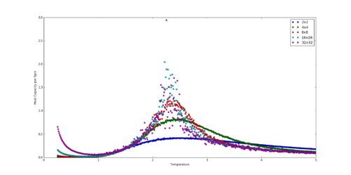
And was created using the following script:

import pylab as pl
import numpy as np
Es = []
VarEs = []
Mgs = []
StdMs = []
absMs = []
StdAbsMs = []
for i in [2,4,8,16,32]:
    print(i)
    temps,energies,energysq,magnetisations,magnetisationsq,aMs = np.loadtxt(str(i) + '_full_200000_with_abs.dat',unpack=True)
    Var_E = (np.array(energysq)-np.array(energies)**2)/i**2
    VarEs.append(Var_E)
fig = pl.figure(figsize=(20,10))
enerax = fig.add_subplot(1,1,1)
enerax.set_ylabel("Heat Capacity per Spin")
enerax.set_xlabel("Temperature")
enerax.plot(temps,np.array(VarEs[0])/temps**2,linestyle='none',marker='o',label='2x2')
enerax.plot(temps,np.array(VarEs[1])/temps**2,linestyle='none',marker='o',label='4x4')
enerax.plot(temps,np.array(VarEs[2])/temps**2,linestyle='none',marker='o',label='8x8')
enerax.plot(temps,np.array(VarEs[3])/temps**2,linestyle='none',marker='o',label='16x16')
enerax.plot(temps,np.array(VarEs[4])/temps**2,linestyle='none',marker='o',label='32x32')
pl.legend(loc='best')
pl.show()

Locating the Curie Temperature

Comparison of Results with Large-Scale Simulation

The per-spin values of $⟨ E ⟩$ , $⟨ E^{2} ⟩$ , $⟨ M ⟩$ , $⟨ M^{2} ⟩$ and $C_{v}$ matched those provided from the C++ simulation well up to and including the $16 \times 16$ lattice (figure 13). The script used is given below.

import pylab as pl
import numpy as np
for i in [2,4,8,16,32]:
    print(i)
    sT,sE,sEsq,sM,sMsq,aMs = np.loadtxt(str(i) + '_full_200000_with_abs.dat',unpack=True)
    bigT,bigE,bigEsq,bigM,bigMsq,bigHc = np.loadtxt(str(i) + 'x' + str(i) + '.dat',unpack=True)
    sHc = (np.array(sEsq)  - np.array(sE) ** 2 )/i**2 * 1 / sT ** 2

    fig = pl.figure(figsize=(20,30))

    enerax = fig.add_subplot(5,1,1)
    enerax.set_ylabel(r'$\langle E \rangle$ per spin')
    enerax.plot(sT,sE/i**2,linestyle = 'none',marker = 'o',label = 'Python')
    enerax.plot(bigT,bigE,linestyle = 'none',marker = 'o',label = 'C++')
    enerax.set_ylim([-2.1, 0])

    esqax = fig.add_subplot(5,1,2)
    esqax.set_ylabel(r'$\langle E^2 \rangle$ per spin')
    esqax.plot(sT,np.array(sEsq)/i**4,linestyle = 'none',marker = 'o')
    esqax.plot(bigT,bigEsq,linestyle = 'none',marker = 'o')

    magax = fig.add_subplot(5,1,3)
    magax.set_ylabel(r'$\langle M \rangle$ per spin')
    magax.set_ylim([-1.2,1.2])
    magax.plot(sT,sM/i**2,linestyle = 'none',marker = 'o')
    magax.plot(bigT,bigM,linestyle = 'none',marker = 'o')

    msqax = fig.add_subplot(5,1,4)
    msqax.set_ylabel(r'$\langle M^2 \rangle$ per spin')
    msqax.plot(sT,sMsq/i**4,linestyle = 'none',marker = 'o')
    msqax.plot(bigT,bigMsq,linestyle = 'none',marker = 'o')

    HCax = fig.add_subplot(5,1,5)
    HCax.set_ylabel(r'$C_{v}$ per spin')
    HCax.plot(sT,sHc,linestyle = 'none',marker = 'o',label = 'Python')
    HCax.plot(bigT,bigHc,linestyle = 'none',marker = 'o',label = 'C++')
    HCax.set_xlabel("Temperature")
    pl.legend(loc='best')
    pl.show()

It is likely that the increasing discrepancy between the two datasets with increasing lattice size arises from a requirement for a large number of steps in order to accurately describe the fluctuations of a larger lattice (which require a larger number of spin flips and thus more spin flips).

Polynomial Fitting

To obtain the position of a maximum in a noisy curve in a more sophisticated manner than visual identification, it is common to resort to curve-fitting.

The fit of a 15th order polynomial to the curve of $C_{v}$ against temperature over the whole temperature range is shown in figure 14, using the following python script:

import numpy as np
import matplotlib.pyplot as plt
temps,energies,energysq,magnetisations,magnetisationsq,Hc = np.loadtxt('64x64.dat',unpack=True)
fit_b = np.polyfit(temps,Hc,15)
plt.figure(figsize=(10,10))
plt.plot(temps,np.polyval(fit_b,temps), label = 'Polynomial fit')
plt.plot(temps,Hc,label='Simulation data',linestyle = 'none', marker = 'o')
plt.xlabel('Temperature')
plt.ylabel(r'$C_{v}$')
plt.legend()
plt.show()

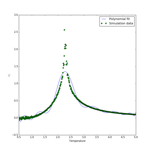
Clearly, the polynomial fit vastly overestimates the width and underestimating the height of the peak. Note how large an order of polynomial was required to achieve at least a moderately good fit, and it was found that further increases in the order did not yield significant improvements.

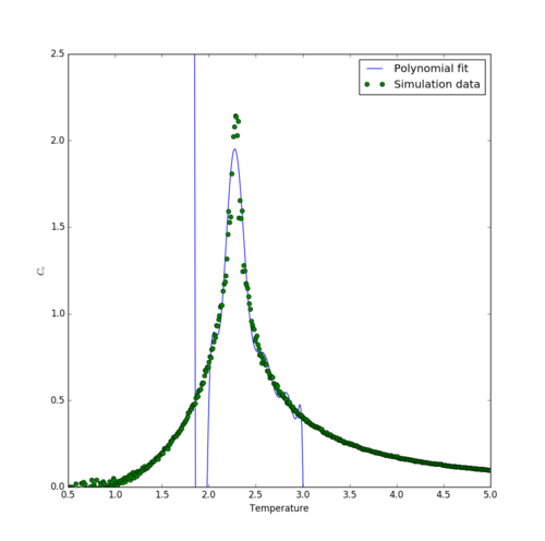
One way of addressing these shortcomings is to only fit the part of the $C_{v}$ that is needed for locating the Curie temperature - namely, the peak. For the same order of polynomial (15), the width and height of the peak is reproduced much more successfully by the fit over only the peak temperature range (figure 15), using the below script:

import numpy as np
import matplotlib.pyplot as plt
temps,energies,energysq,magnetisations,magnetisationsq,Hc = np.loadtxt('64x64.dat',unpack=True)
Tmin = 2
Tmax = 3
sel = np.logical_and(temps>Tmin,temps<Tmax)
PeakValsT = temps[sel]
PeakValsHc = Hc[sel]
fit_b = np.polyfit(PeakValsT,PeakValsHc,15)
plt.figure(figsize=(10,10))
plt.plot(temps,np.polyval(fit_b,temps), label = 'Polynomial fit')
plt.plot(temps,Hc,label='Simulation data',linestyle = 'none', marker = 'o')
plt.xlabel('Temperature')
plt.ylabel(r'$C_{v}$')
plt.ylim([0,2.5])
plt.legend()
plt.show()

Calculating the Curie Temperature

Using the temperature at which $C_{v}$ is at a maximum as an estimate of $T_{C}$ , the Curie temperature of an infinite Ising lattice can be obtained using the scaling relation $T_{C, L} = \frac{A}{L} + T_{C, \infty}$ , where $L$ is the side length of the square Ising lattice. Thus, the relationship between $T_{C, L}$ and $\frac{1}{L}$ is expected to be linear with a constant of $T_{C, \infty}$ .

Using the simulation data provided in the 'C++_data' folder, such a plot, together with the corresponding linear fit, is shown in figure 16. The below script was used to obtain this:

import numpy as np
import matplotlib.pyplot as plt
maxTs = []
invL = 1/np.array([2,4,8,16,32,64])
for i in [2,4,8,16,32,64]:
    temps,energies,energysq,magnetisations,magnetisationsq,Hc = np.loadtxt(str(i) + 'x' + str(i) + '.dat',unpack=True)
    Tmin = 2
    Tmax = 3
    sel = np.logical_and(temps>Tmin,temps<Tmax)
    PeakValsT = temps[sel]
    PeakValsHc = Hc[sel]
    fit_g = np.polyfit(PeakValsT,PeakValsHc,35)
    Tset = np.linspace(Tmin+0.01,Tmax-0.01,1000)
    Hcset = np.polyval(fit_g,Tset)
    maxHc = max(Hcset)
    maxT = Tset[list(Hcset).index(maxHc)]
    maxTs.append(maxT)
plt.figure(figsize=(10,10))
fit_t,cov = np.polyfit(invL,maxTs,1,cov = True)
plt.plot(invL,np.polyval(fit_t,invL),label = str(fit_t[0])+ '/L + ' + str(fit_t[1]))
plt.plot(invL,maxTs,linestyle = 'none', marker = 'o')
plt.ylabel(r'$T_{C}$')
plt.xlabel(r'$\frac{1}{L}$')
plt.legend(loc='best')
print(np.sqrt(cov[1][1]))
plt.show()

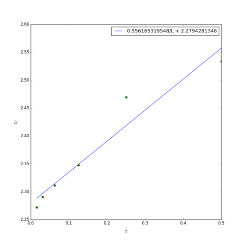
The obtained value of $T_{C, \infty} = 2.28 \pm 0.02$ is within error of the analytical Curie temperature of $\frac{2}{\ln (1 + \sqrt{2})} \approx 2.269$ solved by Lars Onsager ^[4]. This is really quite remarkable, considering that the simulation box was only up to 64 spins wide. Yet the extrapolation of physical properties (such as the Curie temperature) to an infinitely sized system is in excellent agreement with the exact solution. But it is not only in size that the infinite Ising lattice has been heavily simplified - only a miniscule fraction of all accessible states were sampled through the use of the Monte-Carlo algorithm. The fact that, in spite of all this, the simulated data can be used to accurately predict the behaviour of a macroscopic system is truly impressive.

It is important to differentiate between sources of discrepancy between the output of a single simulation and the behaviour of an infinite Ising lattice at identical conditions, and the sources of error in the extrapolated value of $T_{C, \infty}$ . This is because, through use of the previously mentioned scaling relation, we are in fact taking advantage of this discrepancy to predict the behaviour in the limit of $L \to \infty$ (a process which can also be used for many other properties of the system, and is known as finite size scaling). Thus, it seems unreasonable to attribute the finite nature of the simulations to the error in $T_{C, \infty}$ , when this is what allows us to calculate it in the first place.

The largest source of error in this result is therefore likely to be the limited number of data points from which the linear fit is obtained - especially at larger lattice sizes, where the linear trend is more accurately followed. It has been found however, that finite size scaling does not prove to be very accurate in calculating $T_{C, \infty}$ ^[2], and that a much more successful method relies upon computing the cumulant , $U_{L} = 1 - \frac{⟨ M^{4} ⟩_{L}}{3 ⟨ M^{2} ⟩_{L}^{2}}$ ^[5], at each temperature for each lattice side length $L$ , and finding their point of intersection.

Extension - Comparison to Exact Solution

Lars Onsager achieved fame through his exact solution of the infinite two-dimensional Ising lattice^[4]. It is of course also possible to obtain analytic solutions to any $N \times N$ square Ising lattice with periodic boundary conditions. For a $2 \times 2$ lattice, the quantities needed to calculate the heat capacity (in reduced units) are given by ^[2]:

$Z = 2 e^{8 β} + 12 + 2 e^{- 8 β}$

$⟨ E ⟩ = - \frac{1}{Z} [16 e^{8 β} - 16 e^{- 8 β}]$

$⟨ E^{2} ⟩ = \frac{1}{Z} [128 e^{8 β} + 128 e^{- 8 β}]$

Where $β = \frac{1}{T}$ . The constant volume heat capacity per spin is therefore given by $C_{v} = \frac{⟨ E^{2} ⟩ - ⟨ E ⟩}{4 T^{2}}$

As can be seen in figure 17, the simulated data matches this extremely well, further validating the Monte-Carlo algorithm.

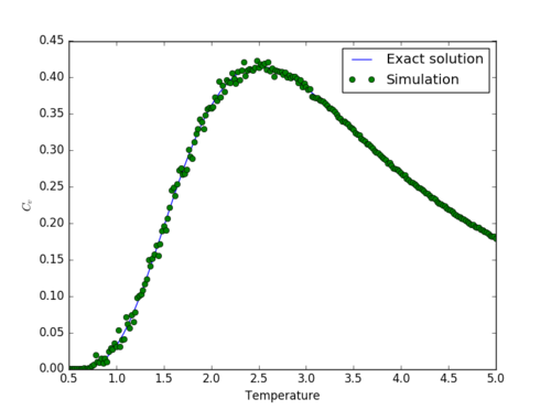
The following code was used to produce figure 17:

import numpy as np
from matplotlib import pyplot as plt
T = np.linspace(0.5,5,1000)
Z = 2*np.exp(8/T) + 12 + 2*np.exp(-8/T)
Es = -1/Z * (2*8*np.exp(8/T)-2*8*np.exp(-8/T))
Esq = 1/Z * (2*64*np.exp(8/T) + 2*64*np.exp(-8/T))
Hcs = (Esq - Es**2)/(4*T**2)
plt.plot(T,Hcs,label='Exact solution')
temps,energies,energysq,magnetisations,magnetisationsq,Hc = np.loadtxt('2x2.dat',unpack=True)
plt.plot(temps,Hc,linestyle = 'none',marker='o',label = 'Simulation')
plt.xlabel('Temperature')
plt.ylabel(r'$C_{v}$')
plt.legend()
plt.show()

References

↑ J. Chem. Phys. 21, 1087 (1953).DOI:10.1063/1.1699114
↑ ^2.0 ^2.1 ^2.2 arXiv:0803.0217 [cond-mat.stat-mech]
↑ American Mathematics Monthly, Vol. 94, (1987), pp. 937-959.
↑ ^4.0 ^4.1 1 L. Onsager, Phys. Rev., 1944, 65, 117–149.DOI:10.1103/PhysRev.65.117
↑ 1 K. Binder, Phys. Rev. Lett., 1981, 47, 693–696.

[1] J. Chem. Phys. 21, 1087 (1953).DOI:10.1063/1.1699114

[arxiv-2] 2.0 ^2.1 ^2.2 arXiv:0803.0217 [cond-mat.stat-mech]

[3] American Mathematics Monthly, Vol. 94, (1987), pp. 937-959.

[Osanger-4] 4.0 ^4.1 1 L. Onsager, Phys. Rev., 1944, 65, 117–149.DOI:10.1103/PhysRev.65.117

[5] 1 K. Binder, Phys. Rev. Lett., 1981, 47, 693–696.

[1]

[2]

[3]

[4]

[5]