Rep:Mod:SohamMgO

Introduction

This lab seeks to investigate phonon-dispersion curves, the free energy and thermal properties of the MgO crystal. This is of vital importance due to the presence of MgO in the Earth’s mantle . In the solid state MgO adopts a face-centred cubic (fcc) Halite structure, similar to NaCl. Lattice dynamics calculation were performed to check correspondence with (mainly) classical theory, and some quantum theory. Finally a molecular dynamics (MD) was performed to contrast with the lattice dynamics calculations.

Computational Methodology

The General Utility Lattice Program (GULP) was used to perform lattice dynamics simulations . All simulations were carried out under a Buckingham interatomic potential and simpler models were devised (where appropriate) to explain results. Shell models were not used at any point due to difficulties in obtaining analytical solutions from the dynamical matrix.

Brief Summary of Lattice Dynamics

In order to understand the phenomena arising from the simulations a model based on a one-dimensional simple monatomic harmonic chain was devised as a first approximation. This model incorporates ideas proposed by Boltzmann , Einstein and Debye. Additional complexity was then added to the model to rationalise the thermal expansion phenomena:

The following dispersion curve that is periodic in k can be obtained for the 1D monatomic linear chain as shown in appendix 1:

• 

• 
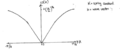  Figure 1 - Dispersion curve for the 1D monatomic chain

This model is in agreement with the Debye model for a solid in so much that the frequency ω varies linearly with k for k→0. But the frequency naturally converges to a maximum at k=π/a, as opposed to the ad hoc ‘cut off’ employed in Debye theory. Another point to note is that this model predicts complete out of phase vibrations at the frequency maxima as can be seen by substitution of k=π/a into the wave ansatz to yield an alternating (-1)ⁿ factor.

The values of k can be shown to be quantised by imposing the periodic boundary condition𝑥_𝑛+𝑁 = 𝑥_𝑛, where N=number of masses in the chain. The physical implication of this condition is that the chain loops round into a circle. This allows all the atoms to be in equivalent environments , and remains valid within the long chain approximation. The wave ansatz is also exposed to the periodic boundary condition: 𝑒^{𝑖𝜔𝑡−𝑖𝑘𝑛𝑎} = 𝑒^{𝑖𝜔𝑡−𝑖𝑘(𝑁+𝑛)𝑎}. Simplifying the wave ansatz gives the restricted values of

$k=\frac{2\pi p}{Na}=\frac{2\pi p}{L},p\in \mathbb{\mathbb{Z}}$

The dispersion relation shows only one value of ω for a given k, implying decoupled oscillations (normal modes). As previously mentioned ω(k) is periodic in k-space (reciprocal space) as well as in real space with periodicity 2π/a. Because transforming k→k+2π yields a physically identical oscillation to the one prior to the transformation, a set of points known as the reciprocal lattice can be defined in k-space that are physically equivalent to the point k=0.Thus k-values only need to be considered in the first Brillouin zone (-π/2 ≤ k ≤ π/2), yielding the total number of normal modes as the ratio between the range of k, and spacing between neighbouring k. This ratio is equivalent to N.

The nearest neighbour forces approximation breaks down in the consideration for MgO. For a diatomic 1D chain the following dispersion relationship can be derived as shown in appendix 2:

• 

• 
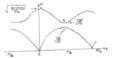  Figure 2- Dispersion curve for 1D diatomic chain displaying the optical branch (top) and acoustic branch (bottom)

This solution ω has two roots- the acoustic branch, and optical branch. By using the small angle approximation in conjunction with the binomial expansion the dispersion relation can be simplified to:

${\omega }^2=\frac{2K(M+m)}{Mm}$

Substitution into the expression for the relative amplitude/ phase correction parameter α (appendix 2) reduces α to two solutions (-M/m, 1). α = -M/m corresponds to point A on Fig. 2, where both masses are oscillating out of phase with the centre of mass (CoM) at rest. The other solution corresponds to the point O, representing long wavelength sound waves (hence the term acoustic branch)

The other limiting case is when ka=π, in which case ω² = (2K/m, 2K/M), corresponding to points (B, C) respectively. In each case only the mass in the expression oscillates and contributes to the frequency. As k→0 on the upper branch, the ions oscillate out of phase to each other and couple strongly to an incident electromagnetic wave (hence the term optical branch). Taking the diatomic model into three dimensions, it can be shown that there are three acoustic branches and three optical branches, and the number of modes associated with each branch is equal to the number of atoms in the unit cell, so there will 3N modes. Therefore it is expected the MgO dispersion will display a total of six (three acoustic and three optic) branches.

Phonon Dispersion Curves

The preceding discussion in modelling lattice vibrations was entirely classical. However the GULP software makes use of quantum mechanics and the model was expanded to allow for quantum phenomena. The condition was imposed that for every normal (defined as a collective oscillation where each mass possesses the same frequency ω) mode of oscillation the corresponding quantum system has energy eigenstates of:

$E_n=\hslash \omega (n+\frac{1}{2})$

Thus, a phonon is defined as a quantum of vibration, with energy ℏ𝜔(𝑘). In the case of an infinite ideal solid there will be an infinite number of phonons. Phonons were calculated by converting the force constant matrix, F, into the dynamical matrix, D. The force constant matrix is obtained using a similar procedure to that used in the lattice dynamics derivation, by approximating it to the second derivative of the potential with respect to the atomic coordinates. But because a solid is being modelled, the terms are multiplied by a corresponding phase factor, thus the force constant matrix between two atoms (i,j) is given by:

$F_i\alpha ,i\beta =\sum _R\frac{{\partial }^{2}U}{\partial \alpha \partial \beta }\bullet exp(ik\bullet (r+R))$

where R=lattice vector within the cut-off radius. The dynamical matrix is defined as

$D=\frac{F}{\sqrt{m_i{m}_j}}$

• 
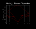  Figure 3- MgO phonon dispersion curve

By calculating their values at point within the Brouillion zone, 3N (or six- as N=2) phonons were recorded per k-point. It can be seen from figure 3 that there is considerable degeneracy near the Γ-point (k=0,0,0), which is indicative of the high symmetry of the crystal. Also all the acoustic modes can be seen to tend towards zero within the same limit. This corresponds to pure translation, and hence zero frequency. This result is also consistent with the definition of wave-vector being inversely proportional to length, and as k → 0, L→∞, and ω ∝ k in the long wavelength limit (with the gradient equal to the sound velocity). Furthermore ω→0 can be justified by the linear coefficient in the Taylor expansion of the potential being zero, because there is not net force at the Γ-point, due to the translational invariance of the infinite crystal:

$\sum _R\mathrm{\nabla }U(R)=0$

In performing this simulation the shell model has been disregarded, because the number of vibrational modes exactly correlates to the number of shells, and so the shell coordinate cannot appear in the D-matrix. There is also a splitting of the optical modes near the Γ-point, and the transverse optical, and longitudinal optical modes are no longer degenerate. This is due to the high charge of the two ions setting up a localised electric field during vibrations in the long-wavelength limit (see appendix 4 for a fuller treatment). Whilst the analytical solution of the D-matrix cannot show this effect, the software employs a correcting factor that incorporates a high frequency dielectric constant tensor ε∞.

• 

Where V=electrostatic potential, q=born effective charge, kΓ = approach to the Γ-point in k-space (which also has an effect on the precise magnitude of splitting). In context, high frequency alludes to the optical frequency by virtue of it being higher than the lattice vibrational frequency.

Phonon DOS calculations

The density of states, g(ω)dω is defined as the number of modes with frequency between ω and ω + dω. Thus it can be defined in 3D as:

• 

In performing the above integral GULP makes use of ‘shrinking factors’ for each reciprocal lattice vector. These specify a point in each direction across the Brillouin zone, and the grid is set so as to maximise the distance from any special points (e.g. the Γ-point since this gives a rapid convergence). The approximation is also made that vibration frequencies are independent of the direction of k. Different grid sizes were sampled to investigate differences in the phonon density of states (DOS):

1x1x1:

• 

2x2x2

• 

3x3x3

• 

4x4x4

• 

The density for the 1x1x1 grid was computed for the point k=0.5 only. This can be readily seen by simply solving the differential equation 𝑔(𝜔)𝑑𝜔=𝑉𝑘²/(2𝜋)³ 𝑑𝑘 , (see appendix 3). Clearly, increasing grid size, gives a smoother function that can eventually be approximated as continuous. A grid size of 3x3x3 was determined to be optimal for the MgO crystal, as van Hove singularities has started to become noticeable in the 4x4x4 grid. These correspond to zone boundaries on the on the dispersion curve (e.g. 400 cm-1, 600 cm-1 etc.). It can be shown that the group velocity can manifest itself in the definition integral of g(ω). This is the source of the singularities as the integral becomes asymptotic as v_g → 0.It can thus be concluded that the optimal grid size depends on the material being modelled (metal, oxide, zeolite etc.), and in particular their lattice structure. The software produces the continuous density function by assigning each phonon into a set range of frequencies and then approximating the curve with theses finite ranges of frequency. It boils down to a compromise between a smaller range in frequency (and hence a better resolution of the curve) and the number of discrete frequency ranges (to maintain a smooth curve)

Thermodynamic features

Several grid sizes were sampled to see how the Helmholtz Free Energy A varies with grid size. Several cubic grids in k-space were sampled, and the free energy was found to converge.

• 
  Figure 4- Helholtz free energy dependence on grid size

The free energy was approximated two have only two contributions, one from the interatomic pair potential, and one from all the vibrational mode. It is suspected that by increasing the grid size, more vibrational modes were surveyed and thus that contribution to the free energy increased. Since the cell size remained constant in both k-space and real space, the system didn’t have access to more vibrational modes, and thus the free energy converged. Therefore the grid size would be independent of the material under study , since the physical cell sample size is not being varied and dictated by the precision/ accuracy required. An example analysis is shown below for the MgO example. The equally spaced ‘mesh’ of k-points given by the shrinking factors are offset from the Γ-point. This is shown to increase the rate of convergence with increasing shrinking factor, as well as avoiding the issue of having to correct for the splitting of the optical branch.

Precision/ meV	Grid Size
1	1x1x1
0.5	2x2x2
0.1	4x4x4

Anharmonic effects

One can model solid state phenomena such as elasticity, and sound velocities by perturbing the ground state of an inter-atomic potential within the simple harmonic approximation with small displacements. However thermal expansion can only be understood by considering the asymmetric part of the potential. However this model is made complicated by introducing coupling of the vibrational modes as a result of considering the anharmonic terms. This coupling can be thought of as the collisions between the phonons associated with those modes. Whilst a phonon will interact with other particles as if it had a momentum ℏ𝑘 (analogous to photons), it cannot carry physical linear momentum because a coordinate in k-space depends on the relative coordinates of the atoms. Thus crystal momentum is defined as a momentum-like vector, which is the momentum modulo the reciprocal lattice. Whilst linear momentum is not conserved in a phonon collision, crystal momentum is. This is a consequence of the fact that translational lattice symmetry is discrete and is therefore ‘exempt’ from Noether’s theorem.

As the amplitude of a vibration is increased (by increasing the temperature), the mean inter-atomic separation of the atoms increases, because the forces are not symmetrical about the equilibrium position. This phenomenon manifests itself macroscopically as thermal expansion. Thermal expansion would not be expected within the harmonic approximation as the mean separation stays constant and so one would expect a constant bond length. The degree towhich a material undergoes thermal expansion can be characterised by the coefficient of thermal expansion α is defined as:

• 

By introducing the bulk modulus B under an isothermal regime as: 𝐵= −𝑉(𝜕𝑝/𝜕𝑉), the thermal expansion coefficient can alternatively be defined as:

• 

Therefore by determining p(T,V), α can be evaluated. The pressure can be determined by consideration of the definition of the Helmholtz Free Energy A, A=U-TS and the fact that 𝑝=−(𝜕𝐴/𝜕𝑉) at constant temperature. The free energy has contributions from the interatomic potential energy, and the free energy associated with each vibration mode, thus the partition function of a single harmonic oscillator is used:

• 

Since the free energy of one vibrational mode is independent of volume, and thus does not contribute to the pressure. And since α is proportional to the pressure gradient with respect to temperature in an isochoric regime there is no contribution to thermal expansion within the harmonic approximation. Therefore within the harmonic limit the following approximations can be made:

• The frequency of vibrations depend on volume
• The total free energy is considered as being the sum of contributions from the interionic potential and vibration modes: A = E_pot + A_{VIB MODES}
• The free energy of each vibration mode is given by:

• 

The algorithm forces the software to stay largely within the harmonic-approximation by assuming harmonic oscillations, but the cell parameters are adjusted to minimise the free energy.Then the pressure is given by:

• 

The Grüneisen parameter γ is introduced in the power law ω ∝ V^-γ which assumes that the volume dependence of all vibrations is independent. Therefore = ∂ω/∂V=-γω/V, and the expression for pressure simplifies to:

• 

And since E_pot is independent of temperature:

• 

where C_V is the heat capacity at constant volume A plot was obtained for the Helmholtz Free Energy dependence on Temperature:

• 

The graph demonstrates the relationship expected, whereby the logarithmic term dominates over the linear term. The lattice vector was also found to increase with temperature- consistent with expansion:

• 

A linear increase could only be modelled with T > 400K. In order to compute the coefficient of it was decided not to attempt determining the Grüneisen parameter from first principles by performing an anharmonic expansion of the potential, but to approximate it within the linear approximation of the volume, the following graph was obtained:

• 

Lattice vector variation with temperature. A very strong empirical fit was determined in the form of y=mx+c. Thus using the parameters ‘m,c’ α could be determined as α=(1/c)*m= 2.650 x 10^-5 K^-1.This is in agreement with a literature value of 1.2 x 10^-5 K^-1 .A consideration of anharmonicity also facilitates the discussion of phase transitions. As MgO approaches its melting point, anharmonicity can cause a mode to vanish, known as a soft mode. At this point the displacement of the molecule becomes time-independent, and the molecule is displaced. This soft mode can be observed with the transverse-optic branch at the Γ-point. As the temperature is cooled through this critical temperature the soft mode can cause the material to display ferro-electric properties.

Finally, the temperature volume dependence through molecular dynamics (MD) simulations was plotted:

• 

The first major difference is that a value cannot be obtained for T→0, since a simulation cannot be run without translational degrees of freedom. This means only the initial value for the lattice parameter is used. Secondly, MD simulations indicate a much smaller value for the volume than lattice dynamics calculations. Thirdly a linear relationship is observed throughout the whole range of temperatures. MD simulations contain full anharmonic effects and display time-correlated results, which lattice dynamic calculations do not. However, since the nuclei are assumed to be classical particles, it fails in the low temperature limit by virtue of it not accounting for quantum effects. This can be combated if a path integral formulation is employed.

Appendix 1- Derivation of the phonon dispersion curve in 1D

• 

Appendix 2- Derivation of the phonon dispersion curve in 2D

• 

Appendix 3- Density of States expression

• 

Appendix 4- Lyddane-Sachs-Teller relation

•