Rep:Mod:RMT CMP

Introduction to the Ising Model

Task 1

The equation

$- \frac{1}{2} J \sum_{i}^{N} \sum_{j \in n e i g h b o u r s (i)} s_{i} s_{j}$

defines the interaction energy between two spins in an Ising Lattice. In the lowest energy configuration, lattice spaces will have the same spin. Each lattice space interacts with its nearest neighbours (not on the diagonal). In one dimension, each lattice space has two nearest neighbours, in two dimensions it has four, and it three dimensions it has six; the number neighbouring spaces for each lattice space is 2 times the number of dimensions. Therefore, each space has $2 D$ interactions, where $D$ is the number of dimensions of the lattice. It doesn't matter whether the spin of the lattice spaces is +1 or -1, as when the interactions are taken into account (multiplied together), the overall interaction energy will always be negative (from the minus sign in the above equation). Iterating through the lattice with $N$ spaces, each space will have $2 D$ interactions. Therefore, $\sum_{i}^{N} \sum_{j \in n e i g h b o u r s (i)} s_{i} s_{j}$ is equal to $2 D N$ . Substituting this back into the original equation gives

$E = - D N J$

As all the lattice spaces in the system described have the same spin, the multiplicity is 2, as all the spins could be pointing up, or they could be pointing down. Multiplicity is related to entropy by the Boltzmann equation: $S = k l n W$ . From this equation, the entropy is calculated* to be $9.57 \times 1 0^{- 24} J K^{- 1}$ .

*Boltzmann constant, k = 1.38 x 10^-23 J K^-1

Task 2

When one of these lattice spaces change spin in a lattice with 3 dimensions and 1000 lattice spaces ( $D = 3, N = 1000$ ), assuming an infinite lattice (periodic boundary conditions), 993 of the lattice spaces are unaffected and would have the same interactions as in the lowest energy state. Each of these individual lattice spaces has six interactions. Assuming the spin of the 999 unchanged spaces to be 1 and the 1 which has flipped to be -1, these 993 lattice spaces would follow the same equation as the ground state energy ( $E = - D N J$ ). The 6 neighbouring spaces to the space with opposite spin have five interactions with spaces with spin 1 and one interaction with spin -1; the overall sum of the spin interactions is 4. The lattice space with opposite spin has 6 neighbouring interactions with a spin opposite to that of itself.

The calculation for this higher state is therefore $- \frac{1}{2} J \times ((993 \times 3) + (6 \times 4) + (- 1 \times 6))$ , which comes out as $- 2988 J$ . The calculation for the lowest energy state, following the equation from the previous section and using the newly defined constants, is $- 3 \times 1000 \times J$ , which comes out as $- 3000 J$ (the units are undefined). Therefore the change in energy of the system when one lattice space changes spin is $+ 12 J$ .

The multiplicity for this new state is 2000; the opposite spin could be in any of the 1000 lattice spaces and the spins could be pointing in one direction, or the other for all of these 1000 possibilities. From the Boltzmann equation, the entropy of the new state is calculated as $1.047 \times 1 0^{- 22} J K^{- 1}$ , and so the change in entropy is calculated to be $9.53 \times 1 0^{- 23} J K^{- 1}$ .

Task 3

From the equation

$M = \sum_{i} s_{i}$

the magnetisation of the one dimensional and two dimensional systems in figure 1 of the wiki script can be calculated. For the 1D system, there are 3 spaces with spin 1 and two spaces with spin -1; $(3 \times 1) + (2 \times - 1) = + 1$ . For the 2D system, there are 13 spaces with spin of 1 and 12 spaces with spin -1; $(13 \times 1) + (12 \times - 1) = + 1$ .

At absolute zero, kinetic energy of the system is at a minimum and so the system would be expected to be in the lowest energy state; all spins are parallel. Therefore, for a system with three dimensions and 1000 lattice spaces, the magnetisation is $\pm 1000$ . At absolute zero, the entropic contributions to the distribution of spin in the system is ignored; it only becomes a factor at higher temperatures.

Calculating the energy and magnetisation

Task 1

Modified code for the energy and magnetisation:

def energy(self):
	energy = 0.0
#the following two loops will loop through each point in the lattice by first looping through the columns and then the rows
	for i in range(self.n_cols):
		for j in range(self.n_rows):
#this is a check for if the point found by the loop is on the edge of the lattice. If it is, the periodic boundary conditions 
#are adhered to by allowing the point to have an interaction with the opposite side of the lattice, as if it were repeating. 
#The energies are then added to to the total energy.
			if i==0:
				energy += -0.5*(self.lattice[j][i]*self.lattice[j][(self.n_cols-1)])
				energy += -0.5*(self.lattice[j][i]*self.lattice[j][i+1])
			elif i==(self.n_cols-1):
				energy += -0.5*(self.lattice[j][i]*self.lattice[j][0])
				energy += -0.5*(self.lattice[j][i]*self.lattice[j][i-1])
			else:
				energy += -0.5*(self.lattice[j][i]*self.lattice[j][i+1])
				energy += -0.5*(self.lattice[j][i]*self.lattice[j][i-1])
			if j==0:
				energy += -0.5*(self.lattice[j][i]*self.lattice[(self.n_rows-1)][i])
				energy += -0.5*(self.lattice[j][i]*self.lattice[j+1][i])
			elif j==(self.n_rows-1):
				energy += -0.5*(self.lattice[j][i]*self.lattice[0][i])
				energy += -0.5*(self.lattice[j][i]*self.lattice[j-1][i])
			else:
				energy += -0.5*(self.lattice[j][i]*self.lattice[j+1][i])
				energy += -0.5*(self.lattice[j][i]*self.lattice[j-1][i])
	return energy

def magnetisation(self):
	magnetisation=0
#again, the following two loops loop through the columns then rows, and then add it onto the final magnetisation in every loop.
	for i in range(self.n_cols):
		for j in range(self.n_rows):
			magnetisation += self.lattice[i][j]
	return magnetisation

Task 2

The picture produced by this code when the number of columns and number of rows were specified in the python terminal and the imported script ILcheck.py was run:

*Figure 1*: Pictures produced by running ILcheck.py

The Curie temperature is the temperature below which a system undergoes spontaneous magnetisation. The picture on the left is the system when it is below the Curie temperature where the entropy contributions are minimised and the energy factor dominates, meaning the spins are all aligned. This represents a ferromagnetic system where all the spins are aligned. The opposite is true for the picture on the right, which represents a diamagnetic system where all the spins cancel out so the overall magnetisation is zero. The picture in the middle shows when entropic and energetic factors are balanced; around the Curie temperature.

Introduction to the Monte Carlo Simulation

Task 1

For a lattice system with 100 lattice spaces (spins), the total number of configurations will be $2^{100}$ . This is because as each lattice space is added to the system, the total number of possible configurations doubles to include all the previous possible configurations with the new spin pointing up, and all the previous configurations with the spin pointing down. This, in standard form, is about $1.27 \times 1 0^{30}$ different configurations. If the computer can calculate $1 \times 1 0^{9}$ configurations, per second, it would take a total of $1.27 \times 1 0^{21}$ seconds to calculate one value of ${⟨ M ⟩}_{T}$ ; clearly far beyond a sensible time.

Task 2

The code for the Monte Carlo cycle:

	def montecarlostep(self, T):
		#the initial energy value is taken from the value calculated in the previous energy function
		energy = self.energy()
		#the following two lines select the coordinates of the random spin which will be flipped
		random_i = np.random.choice(range(0, self.n_rows))
		random_j = np.random.choice(range(0, self.n_cols))
		#the following line flips a random point on the lattice
		self.lattice[random_i][random_j] = -self.lattice[random_i][random_j]
		#the energy for the new lattice is then calculated
		energy_a = self.energy()
		#and the energy difference is calculated
		energy_difference = energy_a - energy
		#the following if statement accepts the new energy if the energy difference is less that zero
		if energy_difference < 0:
			energy = energy_a
		elif energy_difference > 0:
		#the following line chooses a random number in the range[0,1)
		#if the random number is less than or equal to the Boltmann equation, the energy is accepted
		#if not, the lattice is switched back to the original
			random_number = np.random.random()
			if random_number <= np.exp(-energy_difference/T):
				energy = energy_a
			else:
				self.lattice[random_i][random_j] = -self.lattice[random_i][random_j]
		#running totals of the energy and energies squared for the statistics section
		self.E += energy
		self.E2 += energy*energy
		#calculation of the magnetisation for each of the lattices generated using the previously
		#defined magnetisation function
		magnetisation_new = self.magnetisation()
		#running totals for the statistics section
		self.M += magnetisation_new
		self.M2 += magnetisation_new*magnetisation_new
		#running total of the number of cycles the script has run
		self.n_cycles += 1
		return energy, magnetisation_new
	
	def statistics(self):
		#averages for energy and magnetisation
		E_av = self.E/self.n_cycles
		E2_av = self.E2/self.n_cycles
		M_av = self.M/self.n_cycles
		M2_av = self.M2/self.n_cycles
		return E_av, E2_av, M_av, M2_av, self.n_cycles

Task 3

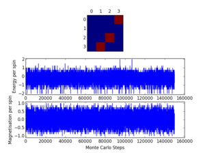
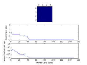
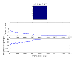
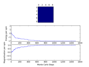
A spontaneous magnetisation may be expected when $T$ is less than $T_{C}$ , the Curie temperature, because below the Cure temperature it becomes energetically favourable for all the spins to allign; the energetic contribution outweighs the entropic contribution. As seen in figure 2, the code has run at below the Curie temperature because there is a spontaneous magnetisation and decrease in energy as the spins align.

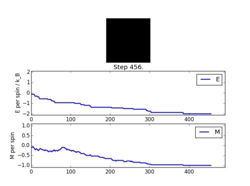
*Figure 2*: Original Monte Carlo code figure displaying the average energy per spin and magnetisation per spin for an 8x8 system

There is a slight delay between the picture and the statistics, as the picture is captured as soon as the save button is clicked, but the statistics are recorded when the window is closed.

Statistics:
Averaged quantities:
E =  -1.42310767591
E*E =  2.27416211354
M =  -0.672441364606
M*M =  0.550456423241
No of cycles =  469

Accelerating the Code

Task 1

Recording how long the code takes to run 2000 steps:

Run 1	19.344911401932038s
Run 2	19.497361657726792s
Run 3	19.28630995568315s
Run 4	19.209311242853204s
Run 5	19.23706365576254s
Run 6	19.214156875098894s
Run 7	19.253119498702148s
Run 8	19.221634150061504s
Run 9	19.27655597194166s
Run 10	19.27494608282649s

Standard Deviation = 0.08012701

Standard Error of Mean (SEM) = 0.025338385

Mean value = 19.2838277273252s ± 0.025338385 (using standard error)

Task 2

Modified code for the energy and magnetisation, using the numpy functions sum, roll and multiply:

	def energy(self):
		#the 0.5 disappears from the formula because the lattice is only 'rolled' once in each direction
                #so the fact that the same interaction could be calculated twice does not need to be considered
		#axis 1 is the vertical axis and axis 0 is the horizontal axis
                #the roll function will move the bottom row to the top row and therefore the periodic boundary conditions are satisfied
		x1 = -np.multiply(np.roll(self.lattice,1,axis=1),self.lattice)
		x0 = -np.multiply(np.roll(self.lattice,1,axis=0),self.lattice)
		energy_x1 = np.sum(x1)
		energy_x0 = np.sum(x0)
		energy = energy_x1 + energy_x0
		return energy

	def magnetisation(self):
		#sums all the elements of the lattice together
		magnetisation=np.sum(self.lattice)
		return magnetisation

Task 3

Recording how long the modified code takes to run 2000 steps:

Run 1	0.146849504551941s
Run 2	0.141200273452888s
Run 3	0.145195445264668s
Run 4	0.142889398112856s
Run 5	0.161044138466600s
Run 6	0.145528423763032s
Run 7	0.162349254532983s
Run 8	0.143811931007320s
Run 9	0.142187235406112s
Run 10	0.142988037291317s

Standard Deviation = 0.00732532

Standard Error of Mean (SEM) = 0.00231647

Mean value = 0.1474043641850s ± 0.00231647

This is a significant decrease in the time taken, showing how much more efficient this new code is, as python can read and process the modified code much quicker.

The Effect of Temperature

Task 1

	Size of the lattice	Temperature	Run Time (number of steps run)	Number of Steps after which the Energy Converges
Test run 1	7x7	1.0	150000	Unable to tell
Test run 2	4x4	1.0	1500	~180-200
Test run 3	4x4	10.0	150000	Unable to tell
Test run 4	4x4	2.5	15000	Unable to tell
Test run 5	4x4	0.5	150	~40-50
Test run 5 repeat	4x4	0.5	150	~40-45

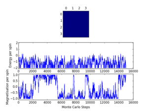
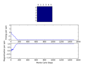
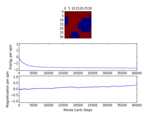
Experimenting with the temperature, it is clear that above T=1.0, it is unclear when the energy converges, so using the data from T=1.0 is much easier in determining how many cycles to ignore. The convergence is also temperature dependent. The following section compares different sizes and the effect of the size of the system on how quickly the energy converges. The repeat of test run 5 shows that rerunning the script with the same conditions gives no real difference in result. However, this may not be the case for all systems because the algorithm is based on random numbers; it could find any stable state (mesostable, as in test run 11 below, or ground state).

	Size of the lattice	Temperature	Run Time (number of steps run)	Number of Steps after which the Energy Converges
Test run 6	6x6	1.0	1500	~150
Test run 7	7x7	1.0	1500	~350-380
Test run 8	8x8	1.0	1500	~800
Test run 9	9x9	1.0	1500	~600-650
Test run 10	10x10	1.0	3000	~1250
Test run 11	32x32	1.0	40000	~10000

Test run 11 shows the largest system encountered by the python scripts in this experiment; 32x32. Modifying the statistics codes to ignore the first 10,000 steps (the number needed in the 32x32 system for the energy to converge) ensures that every system tested does not include the unconverged energies, and also that the same number of energies and magnetisations are used for the averages in all the systems. As the next task runs a code for 150,000 steps, removing 10,000 of these will not make much difference to the overall energy result (only 6.67% of the energies and magnetisations are removed).

The modified code to ignore the first 10,000 steps:

           #defined magnetisation function
		magnetisation_new = self.magnetisation()
                self.n_cycles += 1
		#running totals of the energy and energies squared for the statistics section
		if self.n_cycles > 10000:
			self.E += energy
			self.E2 += energy*energy
		#calculation of the magnetisation for each of the lattices generated using the previously
		
		#running totals for the statistics section
			self.M += magnetisation_new
			self.M2 += magnetisation_new*magnetisation_new
		#running total of the number of cycles the script has run
		return energy, magnetisation_new
	
	def statistics(self):
		#averages for energy and magnetisation
		E_av = self.E/(self.n_cycles-10000)
		E2_av = self.E2/(self.n_cycles-10000)
		M_av = self.M/(self.n_cycles-10000)
		M2_av = self.M2/(self.n_cycles-10000)
		return E_av, E2_av, M_av, M2_av, self.n_cycles

Task 2

The modified code to include the error bars:

enerax.plot(temps, np.array(energies)/spins)
#calculates the standard deviation. The function np.std could also be used
en_stand_dev = np.sqrt(energysq - np.multiply(energies,energies))
#calculated the standard mean error
en_error = np.divide(en_stand_dev,np.sqrt(n_cycles))
#plots the error bars at the data points
enerax.errorbar(temps, np.array(energies)/spins,yerr=en_error,linestyle="None")
magax.plot(temps, np.array(magnetisations)/spins)
mag_stand_dev = np.sqrt(magnetisationsq - np.multiply(magnetisations,magnetisations))
mag_error = np.divide(mag_stand_dev,np.sqrt(n_cycles))
magax.errorbar(temps, np.array(magnetisations)/spins,yerr=mag_error,linestyle="None")

Using the temperature range 0.25 to 5.0 with intervals of 0.25 and 0.1, the following graph was obtained.

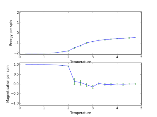
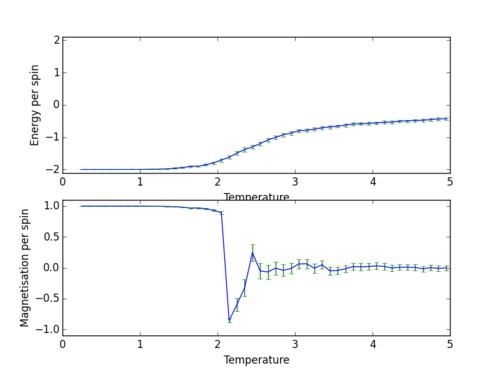
As shown by figure 3 and figure 4, decreasing the size of the temperature interval increases the accuracy and continuity of the graph. For the following section, the interval size was reduced even further to 0.05.

The Effect of System Size

Task 1

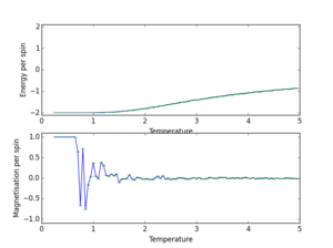
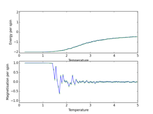
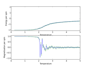
These calculations were run with temperature intervals of 0.05 as this was shown to give a better picture of the shape of the curve without the calculation taking too long.

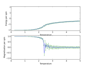
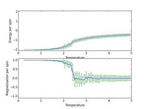
Energy and Magnetisation graphs	Size of the lattice	Run Time (number of steps run)
	2x2	150000
	4x4	150000
	8x8	150000
	16x16	150000
	32x32	150000

Combining all these plots onto the same graph is done by a python script which can be viewed here. The graphs produced are shown below.

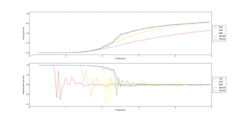
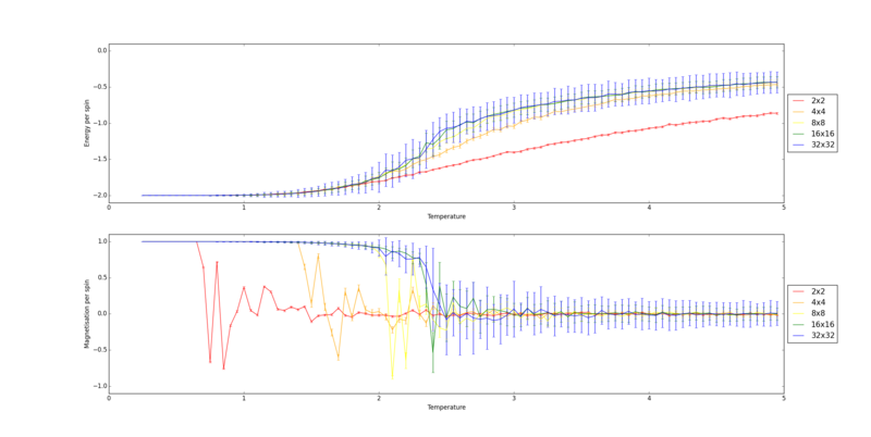
The 32x32 system has the smoothest phase transition with the least fluctuations. However, it can be seen from the above graph that the 16x16 curve is very similar to the 32x32, especially on the energy plot, so it can be assumed that a 16x16 plot is big enough to observe these long range fluctuations. At this point it can be assumed that the size of the system no longer has a strong effect on the energy and magnetisation per spin.

Determining the Heat Capacity

Task 1

Differentiating $C = \frac{\partial ⟨ E ⟩}{\partial T}$ with respect to $T$ :

The expression ${⟨ E ⟩}_{T} = \frac{1}{Z} \sum_{α} E (α) e^{- \frac{E (α)}{k_{B} T}}$ , where $Z (T, N) = {[2 \cosh (\frac{J}{k_{B} T})]}^{N}$ , can be simplified to ${⟨ E ⟩}_{T} = \frac{\sum_{α} E (α) e^{- \frac{E (α)}{k_{B} T}}}{\sum_{α} e^{- \frac{E (α)}{k_{B} T}}}$ . This is because $Z$ is a partition function which defines the total of all the probabilities of the states in the system. $\sum_{α} e^{- \frac{E (α)}{k_{B} T}}$ is just a general form of $Z$ and makes the differential much easier.

${⟨ E ⟩}_{T} = \frac{\sum_{α} E (α) e^{- \frac{E (α)}{k_{B} T}}}{\sum_{α} e^{- \frac{E (α)}{k_{B} T}}} = \sum_{α} E (α) e^{- \frac{E (α)}{k_{B} T}} \times$ $\frac{1}{\sum_{α} e^{- \frac{E (α)}{k_{B} T}}}$ .

For the purpose of making the calculation clearer, the first part of this multiplication will be represented as $x$ and the second part as $y$ .

$x = \sum_{α} E (α) e^{- \frac{E (α)}{k_{B} T}}$

This is differentiated using the chain rule:

$x = \sum_{α} E (α) e^{u}$ $\Rightarrow$ $\frac{\partial x}{\partial u} = \sum_{α} E (α) e^{u}$

$u = - \frac{E (α)}{k_{B} T}$ $\Rightarrow$ $\frac{\partial u}{\partial T} = \frac{E (α)}{k_{B} (T^{2})}$

$\frac{\partial x}{\partial u} \times \frac{\partial u}{\partial T} = \frac{\partial x}{\partial T} = \sum_{α} E (α) e^{u} \times$ $\frac{E (α)}{k_{B} T^{2}} =$ $\frac{\sum_{α} E {(α)}^{2} e^{- \frac{E (α)}{k_{B} T}}}{k_{B} T^{2}}$

$y$ can also be differentiated using the chain rule:

$y = \frac{1}{\sum_{α} e^{- \frac{E (α)}{k_{B} T}}} = u^{- 1}$ $\Rightarrow$ $\frac{\partial y}{\partial u} = - u^{- 2}$

$u = \sum_{α} e^{- \frac{E (α)}{k_{B} T}}$ $\Rightarrow$ $\frac{\partial u}{\partial x} = - \frac{\sum_{α} E (α) e^{- \frac{E (α)}{k_{B} T}}}{k_{B} T^{2}}$

$\frac{\partial y}{\partial u} \times \frac{\partial u}{\partial T} = \frac{\partial y}{\partial T} =$ $- u^{- 2} \times - \frac{\sum_{α} E (α) e^{- \frac{E (α)}{k_{B} T}}}{k_{B} T^{2}} =$ $- \frac{\sum_{α} E (α) e^{- \frac{E (α)}{k_{B} T}}}{k_{B} T^{2} (\sum_{α} e^{- \frac{E (α)}{k_{B} T}})^{2}}$

Using the product rule: $\frac{\partial ⟨ E ⟩}{\partial T} = x y^{'} + x^{'} y = (\sum_{α} E (α) e^{- \frac{E (α)}{k_{B} T}}) (- \frac{\sum_{α} E (α) e^{- \frac{E (α)}{k_{B} T}}}{k_{B} T^{2} (\sum_{α} e^{- \frac{E (α)}{k_{B} T}})^{2}}) + (\frac{\sum_{α} E {(α)}^{2} e^{- \frac{E (α)}{k_{B} T}}}{k_{B} T^{2}}) (\frac{1}{\sum_{α} e^{- \frac{E (α)}{k_{B} T}}})$

Substituting ${⟨ E ⟩}_{T}$ back in gives:

$\frac{\partial ⟨ E ⟩}{\partial T} = - \frac{{⟨ E ⟩}_{T} \times {⟨ E ⟩}_{T}}{k_{B} T^{2}} + \frac{{⟨ E^{2} ⟩}_{T}}{k_{B} T^{2}} = \frac{{⟨ E^{2} ⟩}_{T} - {⟨ E ⟩}_{T}^{2}}{k_{B} T^{2}} = \frac{V a r [E]}{k_{B} T^{2}}$

Task 2

The following script produces a python plot of the heat capacity versus temperature for each of the lattice sizes. Each element has been used in previous codes in the experiment:

 temps2, energies2, energysq2, magnetisations2, magnetisationsq2 = np.loadtxt('2x2.dat',unpack=True)
temps4, energies4, energysq4, magnetisations4, magnetisationsq4 = np.loadtxt('4x4.dat',unpack=True)
temps8, energies8, energysq8, magnetisations8, magnetisationsq8 = np.loadtxt('8x8.dat',unpack=True)
temps16, energies16, energysq16, magnetisations16, magnetisationsq16 = np.loadtxt('16x16.dat',unpack=True)
temps32, energies32, energysq32, magnetisations32, magnetisationsq32 = np.loadtxt('32x32.dat',unpack=True)

en2_hc = np.divide((energysq2 - np.multiply(energies2,energies2)),(np.multiply(temps2,temps2)))
en4_hc = np.divide((energysq4 - np.multiply(energies4,energies4)),(np.multiply(temps4,temps4)))
en8_hc = np.divide((energysq8 - np.multiply(energies8,energies8)),(np.multiply(temps8,temps8)))
en16_hc = np.divide((energysq16 - np.multiply(energies16,energies16)),(np.multiply(temps16,temps16)))
en32_hc = np.divide((energysq32 - np.multiply(energies32,energies32)),(np.multiply(temps32,temps32)))
fig = pl.figure()
pl.ylabel("Heat Capacity")
pl.xlabel("Temperature")
pl.plot(temps2, np.array(en2_hc),color='red',label='2x2')
pl.plot(temps4, np.array(en4_hc),color='orange',label='4x4')
pl.plot(temps8, np.array(en8_hc),color='yellow',label='8x8')
pl.plot(temps16, np.array(en16_hc),color='green',label='16x16')
pl.plot(temps32, np.array(en32_hc),color='blue',label='32x32')
pl.legend(loc='upper left',prop={'size':15})
pl.show()

It produced the following graph:

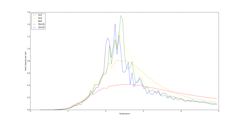
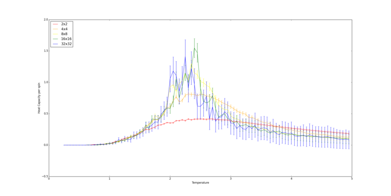
The peaks in the graphs show the approximate location of the Curie temperature. The width of the peak decreases as the system size increases and so as the lattice edge approaches infinity, the width of the peak will become infinitesimally small. This leads to a discontinuity (heat capacity becomes infinity) at the Curie temperature. The shape of the graph is similar to a Boltzmann distribution curve.

Locating the Curie Temperature

Task 1

The following code plots the python data versus the C++ data for energies, energy squared, magnetisations, magnetisation squared and heat capacity. All of the data is plotted per spin. Again all elements of this code has been seen before in this experiment.

from IsingLattice import *
from matplotlib import pylab as pl
import numpy as np

tempsp, energiesp, energysqp, magnetisationsp, magnetisationsqp = np.loadtxt('16x16.dat',unpack=True)
tempsc, energiesc, energysqc, magnetisationsc, magnetisationsqc, heatcapacityc = np.loadtxt('16x16_c+.dat',unpack=True)

var_e = np.subtract(energysqp,np.multiply(energiesp,energiesp))
t_sq = np.multiply(tempsp,tempsp)
heatcapacityp = np.divide(var_e,t_sq)

fig = pl.figure()
enerax = fig.add_subplot(5,1,1)
enerax.set_ylabel("Energy per spin")
enerax.set_xlabel("Temperature")
enersqax = fig.add_subplot(5,1,2)
enersqax.set_ylabel("Energy squared per spin")
enersqax.set_xlabel("Temperature")
magax = fig.add_subplot(5,1,3)
magax.set_ylabel("Magnetisation per spin")
magax.set_xlabel("Temperature")
magsqax = fig.add_subplot(5,1,4)
magsqax.set_ylabel("Magnetisation squared per spin")
magsqax.set_xlabel("Temperature")
hcax = fig.add_subplot(5,1,5)
hcax.set_ylabel("Heat capacity per spin")
hcax.set_xlabel("Temperature")

enerax.plot(tempsp, np.array(energiesp)/256,color='red',label='Python')
enerax.plot(tempsc, np.array(energiesc),color='green',label='C++')
enerax.legend(loc='lower right',prop={'size':12})
enersqax.plot(tempsp, np.array(energysqp)/(256*256),color='red',label='Python')
enersqax.plot(tempsc, np.array(energysqc),color='green',label='C++')
enersqax.legend(loc='lower right',prop={'size':12})
magax.plot(tempsp, np.array(magnetisationsp)/256,color='red',label='Python')
magax.plot(tempsc, np.array(magnetisationsc),color='green',label='C++')
magax.legend(loc='lower right',prop={'size':12})
magsqax.plot(tempsp, np.array(magnetisationsqp)/(256*256),color='red',label='Python')
magsqax.plot(tempsc, np.array(magnetisationsqc),color='green',label='C++')
magsqax.legend(loc='lower right',prop={'size':12})
hcax.plot(tempsp, np.array(heatcapacityp)/256,color='red',label='Python')
hcax.plot(tempsc, np.array(heatcapacityc),color='green',label='C++')
hcax.legend(loc='lower right',prop={'size':12})
pl.show()

The following figure shows the plots for the 16x16 lattice:

There is reasonable similarity in the general shape of the curves but the C++ data has much more fluctuations in the graph and the plot is more continuous. This is due to the fact that the C++ data has many more data points than the python data, therefore giving a more accurate representation of what the curve looks like.

Task 2

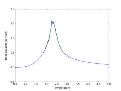
This is the code which tries to fit a polynomial with a specified order to the graph of heat capacity from the C++ data:

from IsingLattice import *
from matplotlib import pylab as pl
import numpy as np

data = np.loadtxt("16x16_c+.dat")
#the variable T takes the first column from the file and C takes the sixth column
T = data[:,0]
C = data[:,5]

#the data is fit to a polynomial here with on order of 31
fit = np.polyfit(T, C, 31)

#the minimum and maximum temperatures are found and then a range of points is generated 
#between them for the x axis
T_min = np.min(T)
T_max = np.max(T)
T_range = np.linspace(T_min, T_max, 1000) 
#the data from the polyfit function is then used to generate a set of points which are an
#approximate fit to the original data over the range of generated temperature points
fitted_C_values = np.polyval(fit, T_range)

#the original data and the fitted data are then plotted together
fig = pl.figure()
pl.ylabel("Heat capacity per spin")
pl.xlabel("Temperature")
pl.plot(T, C)
pl.plot(T_range,fitted_C_values)
pl.show()

The code above is shown only for the 16x16 plot. The fits for all the plots are shown below:

Lattice size	Polynomial order	Graph
2x2	31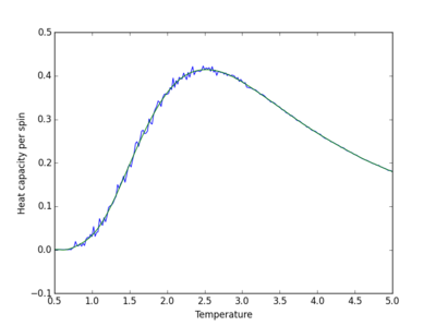
4x4	31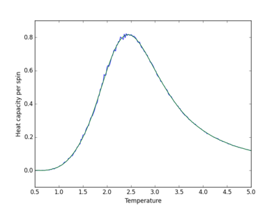
8x8	31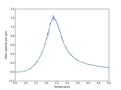
16x16	31
32x32	71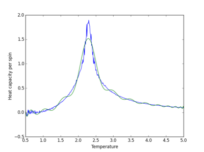
64x64	101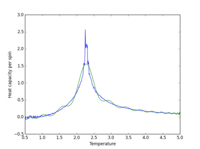

The order of the polynomial used to fit the data is the point when increasing the polynomial no longer improves the fit, and random large fluctuations in the fitted curve appear. Large polynomials are required to produce a suitable fit. The fit becomes more difficult as the system size increases as there are more fluctuations in the curve.

Task 3

The following code improves the fit from the previous task:

from IsingLattice import *
from matplotlib import pylab as pl
import numpy as np

#the following section was seen in the code in the previous section
data = np.loadtxt("16x16_c+.dat")
T = data[:,0]
C = data[:,5]

#the range of temperatures is limited by setting the maximum and minimum temperature
#this fits the curve as best as possible to the peak of the curve
Tmin = 1.8
Tmax = 2.9

selection = np.logical_and(T > Tmin, T < Tmax)
peak_T_values = T[selection]
peak_C_values = C[selection]

#the curve is then fit to, in this case, a polynomial with order 151
fit = np.polyfit(peak_T_values, peak_C_values, 151) 

#a range of values for C are generate over the limited T range
T_min = np.min(peak_T_values)
T_max = np.max(peak_T_values)
T_range = np.linspace(T_min, T_max, 1000) 
fitted_C_values = np.polyval(fit, T_range)

#the graph is then plotted
fig = pl.figure()
pl.ylabel("Heat capacity per spin")
pl.xlabel("Temperature")
pl.plot(T, C)
pl.plot(T_range,fitted_C_values)
pl.show()

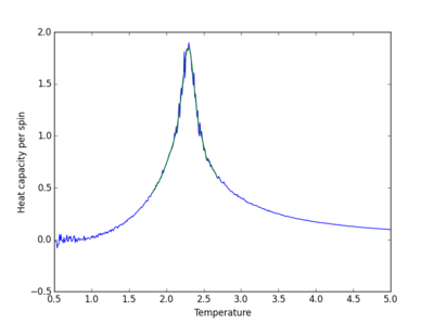
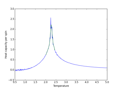
The figure below gives the fitted curve. Again, the code above shows the fit for the 16x16 system. The table blow shows the fit for all the systems:

Lattice size	Polynomial order	Heat capacity at the peak	Temperature at the peak	Range fitted over
2x2	151	0.414234912711	2.52008008	0.5 - 5.0
4x4	151	0.815611319194	2.44418418	0.5 - 5.0
8x8	151	1.20215262144	2.34444444	1.0 - 4.0
16x16	151	1.55985927209	2.31318318	1.8 - 3.0
32x32	101	1.85044080019	2.29272272	1.8 - 2.7
64x64	101	2.21480751038	2.27256256	2.0 - 2.45

This fit is then used in the following section to find the Curie temperature for all the systems tested. The data used is from the C++ tests.

Task 4

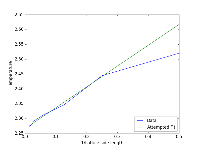
Plotting the data from the previous section in a $\frac{1}{L}$ vs $T$ relationship gives the parameters $A$ and $T_{C, \infty}$ in the equation $T_{C, L} = \frac{A}{L} + T_{C, \infty}$ . The graph shown below is the plot of that data and the attempted fit:

*Figure 10.* The Curie temperature relationship fit to the data obtained from the C++ experiments

When $\frac{1}{L}$ = 0, the side length of the lattice is infinity, hence why the y intercept is equal to $T_{C, \infty}$ . The value of $T_{C, \infty}$ obtained from the fit was $2.2802 \pm 0.0384$ . The inaccurate fit is due to the fact that the graphs for the different lattice sizes are not completely discontinuous at the Curie temperature, which will lead to an error in the result. The experimental exact value for the Curie temperature is $2.269185$ ^[1]. By fitting the data to the four largest systems: 8x8, 16x16, 32x32 and 64x64 (the graph shown below) there is a much better agreement with the experimental Curie temperature: $2.2692 \pm 0.0317$ . This is because of a large error generate from the 2x2 and 4x4 graphs which have a very wide and shallow peak.

*Figure 11.* The same fit as figure 10, but only fitted to the three highest lattice sizes

References

↑ Onsager L. Crystal Statistics. I. A Two-Dimensional Model with an Order-Disorder Transition, Phys. Rev., 1944,65(3-4) p117

[1] Onsager L. Crystal Statistics. I. A Two-Dimensional Model with an Order-Disorder Transition, Phys. Rev., 1944,65(3-4) p117

[1]