
Rep:Mod:PWIN11
COMPUTATIONAL LABS: INORGANIC
Introduction

This report aims to discuss the bonding and structure of several molecules with the aid of computational techniques. Using GaussView 5.0 molecules were modeled from set templates and then optimised using quantum mechanics for further analysis on their physical and chemical properties. High-Performance Computing facility (HPC) was also used to undergo calculations that were otherwise too large for a personal computer. Study of bonding, frequency and molecular orbitals was undergone to investigate the level to which computational techniques can be of use by acquiring very detailed data and precise visual models of different inorganic complexes.
The first part of the report comprises several exercises that involved structure optimisation and analysis of bonding in several inorganic molecules of trigonal planar arrangement with the general formula XY3. As well as this, their IR spectra was predicted and MO analysis was carried out.
The second part of the report is centered around a the different conformational isomers that can result from the dimerisation of AlBrCl2 following this reaction:
2 AlBrCl2 ----> Al2Br2Cl4
In theory five possible isomers exist, but one of them is only accessible in solution.
The aim of the second part is to apply the knowledge acquired during the first exercises and apply them to bigger and more complicated molecules and try to explain their chemical and physical properties from the data.
Part 1
Optimising a molecule of BH3

The structural optimisation of a molecule is based on solving the Schrodinger equation for the electron's position and the overal energies of the atoms. The nuclei of the B and H atoms are given a known position and the equation is solved to give the energy corresponding to this position of the nuclei. The next step would consist on varying the positions of the nuclei and calculating the energy again to see if the given energy is higher or lower. The aim of this is to find the positions for all the nuclei where the energy is the lowest for the given electron configuration.
For BH3, the Gaussian DFT B3LYP method was used and the basis set was 3-21G. These parameters define the set of approximations used for solving the Schrodinger equation and the accuracy specified respectively. The initial distances for the bonds were set to 1.52Å, 1.53Å and 1.54Å.
The optimised molecule can be seen below with the calculated bond angles and bond lengths. All bond lengths have been reported to two decimal places and angles are reported to one decimal place to take into account the relative error level. Figure 1 shows the summary of the Optimisation calculation for BH3. The text included in the dotted line box is a copied fragment of the *.log file that contains the results for the calculation where it can be seen how the forces and the displacement items have converged (i.e. it shows the optimisation has been successful) and the exact bond lengths, bond angles and the dihedral angle reported to up to four decimal places.
      Item               Value     Threshold  Converged?

Maximum Force            0.000220     0.000450     YES

RMS     Force            0.000106     0.000300     YES

Maximum Displacement     0.000919     0.001800     YES

RMS     Displacement     0.000447     0.001200     YES

Predicted change in Energy=-1.672479D-07

Optimization completed.

-- Stationary point found.

                          ----------------------------

                          !   Optimized Parameters   !

                          ! (Angstroms and Degrees)  !

--------------------------                            --------------------------

! Name  Definition              Value          Derivative Info.                !

--------------------------------------------------------------------------------

! R1    R(1,2)                  1.1944         -DE/DX =   -0.0001              !

! R2    R(1,3)                  1.1947         -DE/DX =   -0.0002              !

! R3    R(1,4)                  1.1948         -DE/DX =   -0.0002              !

! A1    A(2,1,3)              119.9983         -DE/DX =    0.0                 !

! A2    A(2,1,4)              119.986          -DE/DX =    0.0                 !

! A3    A(3,1,4)              120.0157         -DE/DX =    0.0                 !

! D1    D(2,1,4,3)            180.0            -DE/DX =    0.0                 !

--------------------------------------------------------------------------------
|
The struccture optimisation of a molecule, both using HPC or Gaussview to calculate it produces a *.log file (readable directly) and a *.chk file (writen in binary). The *.log file for this particular optimisation can be found here.
The summary shown in figure 1 gives a quick insight of the results for the calculation. As mentioned before it reports the type of calculation carried out (an optimisation), the method used (B3LYP, which is a hybrid functional approximation within the density functional theory (DFT) that incorporates both Hartree-Fock (HF) theory and ab initio sources) and the basis set (3-21G, a pople basis set which is one of the most basic basis sets that can be used, making the calculation only take 14 seconds to complete).
The Energy corresponding to this optimisation is also found in the summary in atomic units (1 a. u. = 1 Hartree = 2600 kJ/mol) which is equivalent to -69476.68 kJ/mol. This value is highly dependent on the basis set and method used, therefore any slight change in the parameters would make this value change completely. Another important value is the RMS gradient (gradient of the curve of Potential energy vs. distance) which reflects how well the optimisation is carried out (a value lower than 0.001 indicates a successful optimisation). Finally, the last two numbers reported in the summary can give a better visual idea of the geometry: the point group and the dipole moment. The dipole moment is expected to be zero because the molecule has a trigonal planar arrangement where all three bonds are meant to be equal in length and form three 120° angles, therefore any dipole moment should be cancelled out to zero and the symmetry should correspond to D3h . The reason neither value shows the expected result, is due to the fact that the symmetry was broken when the molecule was created and all three bonds were set at different distances, this could have been corrected by locking the symmetry and selecting the point group manually before the calculation. However, the bond distances in the molecule (to up to 2 dp) and the angles (to up to 1 dp) show a clear correspondence to a D3h symmetry and an almost close to 0 dipole moment.
The theory behind the optimisation process is quite straight forward. When the potential energy of a bond is calculated as a function of the distance between two atoms, a potential energy curve can be drawn. This curve tends to infinity as distance approaches zero, has a minima point and then rises again as distance tends to infinity. The theory behind this is that when the distance between two atoms is too short, the electron-electron repulsion will be too strong and the energy will rise. But when the distance is too big, there is no possibility of having favorable interactions between both atoms causing again the potential energy to rise. It is only at a certain distance where both atoms can experience favorable interactions that overcome the repulsive forces between the atoms and so that the energy is lowered and certain stability is achieved. This is what can be defined as a bond: the stability achieved between two atoms that are close enough to interact favorably (i.e. attractive electrostatic forces) that are strong enough to overcome the unfavorable interactions between the atoms and hold them together. At this minima point, the gradient of the curve is zero, and that is why a good indication of a successful optimisation is whether the nomalised RSM Gradient is zero as it will indicate the lowest energy point of the potential energy curve. All this is important during the optimisation process because when the calculations are carried out, the main objective is to minimise the overall energy and to minimise the gradient.


| Optimisation Step | Total Energy (Hartree) | Norm RSM Gradient (Hartree/Bohr) |
|---|---|---|
| 1 | -26.3666 | 0.0367143 |
| 2 | -26.4031 | 0.0332167 |
| 3 | -26.4561 | 0.0143869 |
| 4 | -26.4622 | 0.00156757 |
| 5 | -26.4622 | 0.00183962 |
| 6 | -26.4623 | 0.000476195 |
| 7 | -26.4623 | 0.000088513 |
The optimisation process can be seen on Gaussian in the form of a graph in figure 3. It can be seen how the overall energy is lower and lower at each optimisation step and how the gradient also tends to zero. The exact values for the energy and the gradient are recorded in table 1. Figure 2 shows the different positions of the nuclei during the process of optimisation. GaussView establishes the existence of a bond based on a set distance criteria, that is why some of the images do not show bonds between the atoms. If however, the existence of a bond is based on the overall favorable energy interaction and stability of a molecule, a bond between B and H could exist at any point of the optimisation steps.
Pseudo-Potentials and Basis Sets
The optimisation of larger molecules can prove to be more challenging. Molecules of the third row of the periodic table and below have a large number of electrons and exhibit relativistic dynamics where valence electrons behave differently to those in the inner core of the atom. Electrons closer to the nucleus are much more tightly bound and shield outer-electrons of the effect of the nucleus. In order to optimise large molecules with a larger number of electrons and molecular orbitals, Pseudo-Potentials and larger basis sets are used to make calculations easier but equally accurate.
Using Pseudo-Potentials involves using an approximation where only the valence electrons (directly involved in the actual bonding of the molecule) are taken into account for the optimisation process and all the inner-core electrons are ignored. The basis set, as mentioned before, is essentially the "accuracy" of this optimisation process. In more precise terms, the basis set is the set of functions used as a linear combination to define the molecular orbitals of the atoms, so the larger number of functions used in this linear combination (a larger basis set) will be able to define molecular orbitals more accurately.
In the following exercise, three trigonal planar molecules were optimised and the results are shown below.
BH3

BH3 was optimised with a 3-21G basis set in the previous section. Here a larger basis set was used and as before, the log file can be found here and the summary of the calculation can be seen in figure 4. As before, The measurements in the log file are shown to up to 4 dp, but the distances shown in the jmol file below are only reported to up to 2 dp for bond distances and to up to 1 dp for the bond angles to account for the relative error.
Several things can be discussed from these results. Firstly, as in the case before, the point group is not D3h for the same reasons and secondly, its is important to mention that although the energies in a. u. seem similar in both optimisation cases, they cannot be compared as different basis set were used.
- Method: B3LYP
- Basis set: 6-31G (d,p)
- Calculation: Optimisation
        Item               Value     Threshold  Converged?
Maximum Force            0.000012     0.000450     YES

RMS     Force            0.000008     0.000300     YES

Maximum Displacement     0.000061     0.001800     YES

RMS     Displacement     0.000038     0.001200     YES

Predicted change in Energy=-1.068331D-09

Optimization completed.

-- Stationary point found.

                          ----------------------------

                          !   Optimized Parameters   !

                          ! (Angstroms and Degrees)  !

--------------------------                            --------------------------

! Name  Definition              Value          Derivative Info.                !

--------------------------------------------------------------------------------

! R1    R(1,2)                  1.1923         -DE/DX =    0.0                 !

! R2    R(1,3)                  1.1923         -DE/DX =    0.0                 !

! R3    R(1,4)                  1.1923         -DE/DX =    0.0                 !

! A1    A(2,1,3)              120.0007         -DE/DX =    0.0                 !

! A2    A(2,1,4)              119.9938         -DE/DX =    0.0                 !

! A3    A(3,1,4)              120.0055         -DE/DX =    0.0                 !

! D1    D(2,1,4,3)            180.0            -DE/DX =    0.0                 !

 --------------------------------------------------------------------------------
GaBr3

For the optimisation of GaBr3, the HPC facility was used. Similarly as before the log file can be accessed here [1] and a summary of the calculation is reported in figure 5.
Besides the fact that a different basis set is used (medium level), the symmetry of the molecule was pre-defined when creating the molecule and this is reflected in the results of the calculations. The point group recorded in this case in the summary table is indeed D3h and the dipole moment is exactly 0.
- Method: B3LYP
- Pseudo Potential: LanL2DZ
- Calculation: Optimisation
         Item               Value     Threshold  Converged?
Maximum Force            0.000000     0.000450     YES

RMS     Force            0.000000     0.000300     YES

Maximum Displacement     0.000002     0.001800     YES

RMS     Displacement     0.000001     0.001200     YES

Predicted change in Energy=-5.834383D-13

Optimization completed.

-- Stationary point found.

                          ----------------------------

                          !   Optimized Parameters   !

                          ! (Angstroms and Degrees)  !

--------------------------                            --------------------------

! Name  Definition              Value          Derivative Info.                !

--------------------------------------------------------------------------------

! R1    R(1,2)                  2.3502         -DE/DX =    0.0                 !

! R2    R(1,3)                  2.3502         -DE/DX =    0.0                 !

! R3    R(1,4)                  2.3502         -DE/DX =    0.0                 !

! A1    A(2,1,3)              120.0            -DE/DX =    0.0                 !

! A2    A(2,1,4)              120.0            -DE/DX =    0.0                 !

! A3    A(3,1,4)              120.0            -DE/DX =    0.0                 !

! D1    D(2,1,4,3)            180.0            -DE/DX =    0.0                 !

--------------------------------------------------------------------------------
BBr3

The log file can be accessed here [2] and a summary of the calculation is reported in figure 6. As in the previous example, the HPC facility was used to undertake the calculations, but the symmetry was not locked.
The basis set in this case is a mixture of a basis set (for B) and the Pseudo Potential (for Br) so the atoms are treated more accurately.
- Method: B3LYP
- Basis set: 6-31(d,p) + LANL2DZ (mixture of basis set and PP)
- Calculation: Optimisation
         Item               Value     Threshold  Converged?

Maximum Force            0.000021     0.000450     YES

RMS     Force            0.000011     0.000300     YES

Maximum Displacement     0.000115     0.001800     YES

RMS     Displacement     0.000063     0.001200     YES

Predicted change in Energy=-2.469464D-09

Optimization completed.

-- Stationary point found.

----------------------------

!   Optimized Parameters   !

! (Angstroms and Degrees)  !

--------------------------                            --------------------------

! Name  Definition              Value          Derivative Info.                !

--------------------------------------------------------------------------------

! R1    R(1,2)                  1.9339         -DE/DX =    0.0                 !

! R2    R(1,3)                  1.934          -DE/DX =    0.0                 !

! R3    R(1,4)                  1.934          -DE/DX =    0.0                 !

! A1    A(2,1,3)              119.9975         -DE/DX =    0.0                 !

! A2    A(2,1,4)              120.0004         -DE/DX =    0.0                 !

! A3    A(3,1,4)              120.0021         -DE/DX =    0.0                 !

! D1    D(2,1,4,3)            180.0            -DE/DX =    0.0                 !

--------------------------------------------------------------------------------
Structure Comparison
| BH3 | BBr3 | GaBr3 | |
|---|---|---|---|
| Bond Length (Å) | 1.19 | 1.93 | 2.35 |
| Literature Value Bond Length (Å) | 1.19[3] | 1.90[4] | 2.38[5] |
Table 2 shows the bond lengths calculated from the structure optimisation of the three molecules. The values obtained have been compared to literature values and it is clear how the results are in good agreement with the obtained bond lengths. The relative error resulting from the different calculations is of ±0.01Å.
As mentioned before, a bond can be considered the favorable interaction between two atoms which is overall attractive which holds the overall structure. This favorable interaction is a delicate balance between the molecular energies and the electrostatic forces acting on the atoms and particles. This means, that if the distance is too short, the electrostatic interactions of repulsive nature between electrons will cause the energy to rise drastically but a distance between the two atoms too large will not allow positive interaction between the molecular orbitals and therefore the energy will rise again. This ideal distance is defined as the atomic covalent radii, and it can be a useful tool to predict bond lengths.
The effect of different centers at the trigonal planar structure and the effect of different ligand molecules can be compared with these three complexes. The bonding model for BX3 molecules is based on a B center of coordination III that forms three covalent bonds with three 1 electron donor ligands. Both H and Br require 1 electron to complete their outermost shell and acquiring the stability associated to a full orbital. At first glance, it is clear that H, having a much smaller atomic radii than Br should form smaller bonds distances. H electronic configuration is [H] = 1s1 (valence electron located on 1st shell) and Br electronic configuration is [Br] = [Ar] 4s2 3d10 4p5 (valence electrons located on 4th shell). The covalent bond lengths can be predicted by adding both covalent radii of each atom:
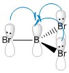
The predicted covalent bond length for B-H is quite accurate (Δ (Å)= 0.03), the B-Br bond however suffers a more significant deviation from the predicted covalent bond length (Δ (Å)= 0.11). This is due to the possible electron donation of the lone pairs of the Br into the empty pz orbital on the Boron atom. Its planar geometry allows a good overlap between the lone pair located on the halide pz orbital and the central B empty orbital as seen in figure 7, lowering its energy and making the bond stronger and therefore shorter. The strength of this molecular orbital overlap depends on the relative orientation of the orbitals, their relative size and their relative energies. Because Br is a large atom compared to B, its molecular orbitals are larger and more diffused, therefore the overlap is not ideal so the effect is small. However it is important enough to show a shorter covalent bond to the one predicted. This empty orbital on the metal center is what makes BX3 complexes such good Lewis acids.
For complexes with different atom centers but with same ligands, BBr3 and GaBr3 are compared. As before, the nature of the bonds is covalent, and we can predict the bond length by adding the covalent radii:
The difference of the predicted to the calculated bond length for Ga-Br (Δ (Å)= 0.07)is also quite high. Again, the main reason for this will be lone pair donation into the empty pz orbital of the metal center, that cannot occur with the B-H bond as no lone pair exist to donate electron density. The reason why this electron donation is weaker than with B-Br can be due to the fact that even though the orbitals are now similar in size (both atoms are fourth row elements), the orbitals are very diffused spreading the electron density over a larger area and therefore making the interaction weaker.
Frequency analysis
Frequency analysis is another interesting feature that can be predicted and analysed with computational techniques. Vibrational analysis is complementary to the optimisation of molecule structures. The gradient of a potential energy curve will allow us to determine the existence of a stationary point, however it is the second derivative of this curve that sheds information on the nature of this stationary point: a minimum would show a ground state configuration whilst a maximum point shows a transition state structure.
A molecule with N atoms has 3N degrees of freedom. The motion of a molecule can be translational (in 3 directions along the 3 axes), rotational (in 3 directions for non-linear molecules) and vibrational. Therefore, if we take into account that XY3 molecules will have 3 rotation motions and 3 translation motions, there is 3(N)-6 = 3x(4)-6 = 6 vibration modes.
Gaussview can also be used to animate these vibrations and observe the actual frequency motions of the molecules.
Vibrational modes can be assigned symmetry labels that can be predicted from the point group theory by treating the vibrational modes like molecular orbitals or they can be calculated by Gaussview. This labeling can be very useful to easily predict allowed of forbidden electronic transition, dipole moment or IR visible vibrational modes. Degenerate modes of vibrations have the same energy and can be transformed into each other by symmetry operations.
BH3

For the frequency analysis, a molecule of BH3 was created and then optimised but its point group was manually set to D3h. The calculation for the vibrational analysis was then carried out on Gaussian. The reason for setting the symmetry is that better results are generated. It is very complicated to manually adjust the bond lengths with Gaussview so by locking the point group, we ensure the correct symmetry for the molecule.
- Method: B3LYP
- Basis set: 6-31G (d,p)
- Calculation: Frequency
The summary of the calculation is depicted in figure 8, the log file can be found here. The fragment from the log file copied below shows a fragment that can give an idea of the accuracy of the results obtained. The rotational and translational frequencies can be found in the first line of "low frequencies" seen in the *.log file. The six expected vibration modes can be seen below and they are recorded in table 3. Two of the vibration modes are doubly degenerate and two a singly degenerate. Finally, fig.9 is the predicted IR spectra for a BH3 molecule. Not all vibration modes can be seen as peaks in the spectra, the intensity for IR spectroscopy depends on the change of the dipole moment during the vibration whereas for RAMAN spectroscopy, the intensity depends on the polarizability. Of the 6 modes of vibrations observed: A1’ (Raman Active), 2E’(IR + Raman Active), A2’’(IR Active).
Low frequencies ---   -2.9884   -1.1079   -0.0055    1.6554    9.9523   10.0137
Low frequencies --- 1162.9840 1213.1744 1213.1770

Diagonal vibrational polarizability:

0.7180863       0.7179861       1.8414489

Harmonic frequencies (cm**-1), IR intensities (KM/Mole), Raman scattering

activities (A**4/AMU), depolarization ratios for plane and unpolarized

incident light, reduced masses (AMU), force constants (mDyne/A),

and normal coordinates:

                       1                      2                      3

                       A2"                    E'                     E'

Frequencies --   1162.9840              1213.1744              1213.1770

Red. masses --      1.2531                 1.1072                 1.1072

Frc consts  --      0.9986                 0.9601                 0.9601

IR Inten    --     92.5495                14.0546                14.0582

Atom  AN      X      Y      Z        X      Y      Z        X      Y      Z

1   5     0.00   0.00   0.16     0.00   0.10   0.00    -0.10   0.00   0.00

2   1     0.00   0.00  -0.57     0.00   0.08   0.00     0.81   0.00   0.00

3   1     0.00   0.00  -0.57     0.39  -0.59   0.00     0.14  -0.39   0.00

4   1     0.00   0.00  -0.57    -0.39  -0.59   0.00     0.14   0.39   0.00

                       4                      5                      6

                      A1'                    E'                     E'

Frequencies --   2582.3193              2715.4935              2715.4946

Red. masses --      1.0078                 1.1273                 1.1273

Frc consts  --      3.9596                 4.8978                 4.8979

IR Inten    --      0.0000               126.3287               126.3191

Atom  AN      X      Y      Z        X      Y      Z        X      Y      Z

1   5     0.00   0.00   0.00     0.11   0.00   0.00     0.00   0.11   0.00

2   1     0.00  -0.58   0.00     0.02   0.00   0.00     0.00  -0.81   0.00

3   1     0.50   0.29   0.00    -0.60  -0.36   0.00    -0.36  -0.19   0.00

4   1    -0.50   0.29   0.00    -0.60   0.36   0.00     0.36  -0.19   0.00

| Vibr. Mode | Motion | Dipole Derivative unit vector | Description of Motion | Freq (cm-1) | IR Intensity (KM/mol) | ε (10-40 esu2 cm2) | D3h point group |
|---|---|---|---|---|---|---|---|
| 1 (ν2) |  
|

|
Concerted wagging motion of the 3H atoms. Singly degenerate vibrational mode. | 1162.98 | 92.5495 | 317.474 | A2” |
| 2 (ν4) |  
|

|
Scissoring motion of 2H atoms along horizontal plane and consequent B and other H atom motion in opposite direction. 2/3 are doubly degenerate vibrational modes | 1213.17 | 14.0546 | 46.2171 | E’ |
| 3 (ν4) |  
|

|
Assymetric rocking motion of all 3H atoms on the horizontal plane. Small vibration of B. | 1213.18 | 14.0582 | 46.2288 | |
| 4 (ν1) |  
|

|
Symetric stretching motion of 3H atoms on the horizontal plane. B atom remains motionless. Singly degenerate vibration mode. | 2582.32 | 0.0000 | 0 | A1’ |
| 5 (ν3) |  
|
|
Antysymmetric stretch vibration mode of 2H atoms, and small vibratin motion of B atom. 1 of the H atoms remains motionless. 5/6 vibration modes are doubly degenerate. | 2715.49 | 126.3287 | 185.593 | E’ |
| 6 (ν3) |  
|

|
Symmetric stretch vibration mode for 2 of the H atoms and antisymmetric stretch vibration mode of the other H with respect to them. B atom also vibrates. | 2715.49 | 126.3191 | 185.578 |
GaBr3

GaBr BH3 frequency analysis was undergone using the HPC facility. The symmetry had already been locked when the optimisation was done, therefore the same optimised *.log file was submitted into the HPC and the results *.log file can be viewed here[7].
- Method: B3LYP
- Basis set: 6-31(d,p) + LANL2DZ (mixture of basis set and PP)
- Calculation: Frequency
The basis set used was the same as during the optimisation. The reason for this is that all the results especially energy results, are highly dependent on the basis set used, therefore all the comparisons are futile unless it is the same molecule and the basis set is the same. The summary of the calculation is depicted in figure 10.
As before, of the 6 modes of vibrations observed: A1’ (Raman Active), 2E’(IR + Raman Active), A2’’(IR Active). The predicted IR spectra is shown in figure 11
Low frequencies ---   -0.5252   -0.5247   -0.0024   -0.0010    0.0235    1.2010
 Low frequencies ---   76.3744   76.3753   99.6982
 Diagonal vibrational polarizability:
       30.7937168      30.7942540      24.9520712
 Harmonic frequencies (cm**-1), IR intensities (KM/Mole), Raman scattering
 activities (A**4/AMU), depolarization ratios for plane and unpolarized
 incident light, reduced masses (AMU), force constants (mDyne/A),
 and normal coordinates:
                      1                      2                      3
                     E'                     E'                     A2"
 Frequencies --     76.3744                76.3753                99.6982
 Red. masses --     77.4211                77.4212                70.9513
 Frc consts  --      0.2661                 0.2661                 0.4155
 IR Inten    --      3.3447                 3.3447                 9.2161
  Atom  AN      X      Y      Z        X      Y      Z        X      Y      Z
     1  31    -0.39   0.00   0.00     0.00   0.39   0.00     0.00   0.00   0.89
     2  35     0.63   0.00   0.00     0.00   0.41   0.00     0.00   0.00  -0.26
     3  35    -0.15  -0.45   0.00     0.45  -0.37   0.00     0.00   0.00  -0.26
     4  35    -0.15   0.45   0.00    -0.45  -0.37   0.00     0.00   0.00  -0.26
                      4                      5                      6
                     A1'                    E'                     E'
 Frequencies --    197.3371               316.1825               316.1863
 Red. masses --     78.9183                72.2067                72.2066
 Frc consts  --      1.8107                 4.2531                 4.2532
 IR Inten    --      0.0000                57.0704                57.0746
  Atom  AN      X      Y      Z        X      Y      Z        X      Y      Z
     1  31     0.00   0.00   0.00     0.82   0.00   0.00     0.00   0.82   0.00
     2  35     0.00   0.58   0.00    -0.01   0.00   0.00     0.00  -0.47   0.00
     3  35    -0.50  -0.29   0.00    -0.35  -0.20   0.00    -0.20  -0.12   0.00

     4  35     0.50  -0.29   0.00    -0.35   0.20   0.00     0.20  -0.12   0.00

| Vibr. Mode | Motion | Dipole Derivative unit vector | Description of Motion | Freq (cm-1) | IR Intensity (KM/mol) | ε (10-40 esu2 cm2) | D3h point group |
|---|---|---|---|---|---|---|---|
| 1 (ν4) |  
|

|
Asymmetric rocking motion of one H atom and symmetrical rocking of the other 2H atoms. Small vibration of the central B atom. 1 and 2 are doubly degenerate vibration modes. | 76.37 | 3.3447 | 174.71 | E' |
| 2 (ν4) |  
|

|
Scissoring motion of two H atoms and consequent B and other H atom motion in opposite direction. | 76.38 | 3.3447 | 174.707 | |
| 3 (ν2) |  
|

|
Symmetric wagging motion all three H atoms. Small vibration of B. It is a singly degenerate mode. | 99.70 | 9.2161 | 368.78 | A2” |
| 4 (ν1) |  
|

|
Symmetric stretching motion of three H atoms along the horizontal plane. B atom remains motionless. Singly degenerate vibration mode. | 197.34 | 0.0000 | 0 | A1’ |
| 5 (ν3) |  
|

|
Anti-symmetric stretch vibration mode of two H atoms, and small vibration motion of B atom. One of the H atoms remains motionless. 5 and 6 vibration modes are doubly degenerate. | 316.18 | 57.0704 | 720.079 | E’ |
| 6 (ν3) |  
|

|
Symmetric stretch vibration mode for two of the H atoms and anti-symmetric stretch vibration mode of the other H with respect to them. B atom also vibrates. | 316.19 | 57.0746 | 720.124 |
Vibrational Comparison
| Vibr. Mode | BH3
Freq (cm-1) |
GaBr3
Freq (cm-1) |
BH3
IR Intensity (KM/mol) |
GaBr3
IR Intensity (KM/mol) |
D3h point group |
|---|---|---|---|---|---|
| ν1 | 2582.32 | 197.34 | 0.0000 | 0.0000 | A1’ |
| ν2 | 1162.98 | 99.70 | 92.5495 | 9.2161 | A2” |
| ν3 | 2715.49 | 316.18 | 126.3287 | 57.0704 | E’ |
| ν3 | 2715.49 | 316.19 | 126.3191 | 57.0746 | E’ |
| ν4 | 1213.17 | 76.37 | 14.0546 | 3.3447 | E' |
| ν4 | 1213.18 | 76.38 | 14.0582 | 3.3447 | E' |
The comparison of both frequency analysis is quite straightforward. Both the differences and the similarities can be deduced by inspection of the results.
The frequency of a bond is dependent on , where c is the speed of light, k is the force constant (proportional to the strength of the bond) and μ is the reduced mass (). The reduced mass for both bonds are: μB-H = 0.91 and μGa-Br = 37.23. The frequency for the B-H bond vibration modes will therefore be much stronger than the frequency of Br-Ga bond. As well as this, the force constant of the bonds which is proportional to the actual bond strength will also affect the stregth of the frequency. As mentioned before, electron donation occurs from the Br lone pair into the empty pz Ga orbital, so the Ga-Br bond is stronger than would be expected. However, bond dissociation enthalpies show that the B-H bond is much stronger than the Ga-Br bond, which corroborates the data in the tables.
- Bond dissociation energy (298K): Ed(BH2-H) = 106.6 kcal/mol[8]
- Bond dissociation energy (298K): Ed(GaBr2-Br) = 72.18 kcal/mol (302 Kj/mol[9])
The intensity of the frequency peaks, is proportional to the change of dipole moment during the vibration. The derivative of the dipole moment (i.e. the change of the dipole moment) can be seen represented on the molecule as a unit vector. The electronegativity difference between H-B is much larger than Ga-Br, so the change of dipole moment will be more significant for B-H and therefore intensity of the peaks will also be larger. For the vibrations where no dipole change is observed, neither molecule show a peak in the IR spectra.
Another observable difference is the reordering of the vibrational modes. The doubly degenerate v4 mode is actually stronger than the v2 mode for GaBr3 (unlike for BH3). The explanation for this interchange is again because of the reduced mass and the force constant, the only parameters that change in the equation for the frequency.
BH3 Molecular Orbitals
The optimised structure of BH3 can be used to generate the Molecular Orbitals (MOs). Using the 6-31(d,p) basis set, the calculation was undergone using the HPC facility. The log file can be accessed here[10].
By using molecular orbital theory, a MO diagram can be predicted as seen in figure 12.

The MOs calculated with Gaussian are recorded in the table below (the Cartesian coordinates are the same as those used in picture 12).
| 1 (-6.77213 a.u.) | 2 (-0.51218 a.u.) | 3 (-0.35058 a.u.) | 4 (-0.35055 a.u.) |
|---|---|---|---|

|

|

|

|
| 5 (-0.06614 a.u.) | 6 (0.16738 a.u.) | 7 (0.17872 a.u.) | 8 (0.17876 a.u.) |

|

|

|

|
MO Theory allows a new interpretation of bonds based on the linear combination of atomic orbitals (AO). First thing that can be observed is that for the prediction of the MO diagram, only 7 MOs can be seen, however the calculation shows a larger number of MOs. When applying MO theory, only non-core orbitals are taken into account. The MO corresponding to 1, is in fact the very low lying 1s B orbital that does not interact with any of the H orbitals due to the energy difference. It is, of course full and low in energy therefore it does not intervene in any bonding interactions. The calculation for the BH3 MOs, also shows up to 30 MOs predicted. This is in fact the Basis set including combination of B d orbitals. These are also disregarded for our MO diagram.
The last thing that can be mentioned is the great deal of detail that MO calculation can offer. The MOs reflect how higher molecular orbitals tend to be more diffused and larger, as can be seen in the images in table 11. The also show very clearly nodal planes, where different phase orbitals are in close range therefore raising the overall energy. MOs with a larger number of nodal planes and more diffused orbitals are higher in energy.
The relative energy of the MOs can be calculated too by the Gaussian program, they are also reported on the table 11.
NH3: NBO analysis
Natural Bonding Orbitals are molecular orbitals with the highest electron density and they reflect the charge distribution in a molecule.
NH3 was created, optimised using a 6-31(d,p) basis set (view log file here) and the frequency was also analysed to assure that the lowest energy configuration had been found (log file here).
NH3 |

         Item               Value     Threshold  Converged?

Maximum Force            0.000005     0.000450     YES

RMS     Force            0.000003     0.000300     YES

Maximum Displacement     0.000010     0.001800     YES

RMS     Displacement     0.000007     0.001200     YES

Predicted change in Energy=-7.830784D-11

Optimization completed.
Low frequencies ---  -11.6527  -11.6490   -0.0048    0.0333    0.1312   25.5724
Low frequencies --- 1089.6616 1694.1736 1694.1736
As seen above, the energies and the displacements have converged and there are no negative frequencies. the Optimisation process has been successful. In order to carry out the NBO analysis, the MO also have to be calculated. (Log file here). Table 7 summarises the results.
| 1 (-14.30568 a.u.) | 2 (-0.84466 a.u.) | 3 (-0.45030 a.u.) | 4 (-0.45030 a.u.) |
|---|---|---|---|

|

|

|

|
| 5 (-0.25317 a.u.) | 6 (0.07985 a.u.) | 7 (0.16923 a.u.) | 8 (0.16923 a.u.) |

|

|

|

|

Finally, the NBO analysis can be carried out (The log file is the same resulting from the MO calculations). Figure 14 shows the overall charge distribution and the calculated charges. N, as expected holds the most negative charge (-1.125) whilst H is mostly where the positive charge resides (0.375). Overall, the molecule charge of the molecule is zero.
The charge limits associated with the color range for the NBO representation is from -1.000 to +1.000.
The NBO analysis in the *.log file can be found after the MO analysis:
 ******************************Gaussian NBO Version 3.1******************************
N A T U R A L   A T O M I C   O R B I T A L   A N D

N A T U R A L   B O N D   O R B I T A L   A N A L Y S I S

******************************Gaussian NBO Version 3.1******************************

/RESON  / : Allow strongly delocalized NBO set

Analyzing the SCF density
Job title: NH3 MO
Summary of Natural Population Analysis:

Natural Population

               Natural  -----------------------------------------------

Atom  No    Charge         Core      Valence    Rydberg      Total

-----------------------------------------------------------------------

N    1   -1.12515      1.99982     6.11104    0.01429     8.12515

H    2    0.37505      0.00000     0.62249    0.00246     0.62495

H    3    0.37505      0.00000     0.62249    0.00246     0.62495

H    4    0.37505      0.00000     0.62249    0.00246     0.62495

=======================================================================

* Total *    0.00000      1.99982     7.97852    0.02166    10.00000
The natural population analysis shows the overall charge distribution at each atom and respectively in their core, valence and Rydberg orbitals. The overall charge distribution has been summarised in figure 14.
       (Occupancy)   Bond orbital/ Coefficients/ Hybrids
---------------------------------------------------------------------------------

1. (1.99909) BD ( 1) N   1 - H   2

            ( 68.83%)   0.8297* N   1 s( 24.87%)p 3.02( 75.05%)d 0.00(  0.09%)

                                    0.0001  0.4986  0.0059  0.0000  0.0000

                                    0.0000  0.8155  0.0277 -0.2909  0.0052

                                    0.0000  0.0000 -0.0281 -0.0087  0.0013

            ( 31.17%)   0.5583* H   2 s( 99.91%)p 0.00(  0.09%)

0.9996  0.0000  0.0000 -0.0289  0.0072

2. (1.99909) BD ( 1) N   1 - H   3

            ( 68.83%)   0.8297* N   1 s( 24.87%)p 3.02( 75.05%)d 0.00(  0.09%)

                                    0.0001  0.4986  0.0059  0.0000 -0.7062

                                    -0.0240 -0.4077 -0.0138 -0.2909  0.0052

                                    0.0076  0.0243  0.0140  0.0044  0.0013

            ( 31.17%)   0.5583* H   3 s( 99.91%)p 0.00(  0.09%)

0.9996  0.0000  0.0250  0.0145  0.0072

3. (1.99909) BD ( 1) N   1 - H   4

            ( 68.83%)   0.8297* N   1 s( 24.87%)p 3.02( 75.05%)d 0.00(  0.09%)

                                    0.0001  0.4986  0.0059  0.0000  0.7062

                                    0.0240 -0.4077 -0.0138 -0.2909  0.0052

                                    -0.0076 -0.0243  0.0140  0.0044  0.0013

            ( 31.17%)   0.5583* H   4 s( 99.91%)p 0.00(  0.09%)

                                    0.9996  0.0000 -0.0250  0.0145  0.0072

4. (1.99982) CR ( 1) N   1           s(100.00%)

                                     1.0000 -0.0002  0.0000  0.0000  0.0000

                                     0.0000  0.0000  0.0000  0.0000  0.0000

                                     0.0000  0.0000  0.0000  0.0000  0.0000

5. (1.99721) LP ( 1) N   1           s( 25.38%)p 2.94( 74.53%)d 0.00(  0.10%)

                                     0.0001  0.5036 -0.0120  0.0000  0.0000

                                     0.0000  0.0000  0.0000  0.8618 -0.0505

                                     0.0000  0.0000  0.0000  0.0000 -0.0310
Above is the main listing of the NBOs. In this case we find 3 BD (2-center bond), 1 CR (1-center core pair) and a LP (1 lone pair). For the BDs, the amount of charge in each atom (in form of a percentage) is also reported. As expected, most of the charge lies towards the N atom because of it's higher electronegativity. Not only the distribution of the charge in the molecule, but the distribution of the electron density in each orbital on each atom can also be seen, again in the form of a percentage. From this we can tell that the N atoms has essentially 4 sp bonds (±75%p and ±25%s orbitals), three for the N-H bonds and one where the electron density of lone pair is concentrated. The CR NBO is the core 1s electrons located in the N atom that are found completely bound to the N and are not dispersed or interacting with no other orbitals. The number of electrons located in each NBO can be seen in the occupancy, all BD, CR and LP NBO have an occupancy of ≈2 (they are full).
Second Order Perturbation Theory Analysis of Fock Matrix in NBO Basis

Threshold for printing:   0.50 kcal/mol

                                                                          E(2)  E(j)-E(i) F(i,j)

Donor NBO (i)                     Acceptor NBO (j)                       kcal/mol   a.u.    a.u.

===================================================================================================

within unit  1

5. LP (   1) N   1                / 16. RY*(   1) H   2                    1.01    1.43    0.034

5. LP (   1) N   1                / 17. RY*(   2) H   2                    0.67    2.17    0.034

5. LP (   1) N   1                / 20. RY*(   1) H   3                    1.01    1.43    0.034

5. LP (   1) N   1                / 21. RY*(   2) H   3                    0.67    2.17    0.034

5. LP (   1) N   1                / 24. RY*(   1) H   4                    1.01    1.43    0.034

5. LP (   1) N   1                / 25. RY*(   2) H   4                    0.67    2.17    0.034
This section shows the interaction of bonding-antibonding orbitals. All the values in the E(2) column are quite low, which means that there are no major bond-antibond interaction in NH3.
 Natural Bond Orbitals (Summary):

                                                            Principal Delocalizations
            NBO                        Occupancy    Energy   (geminal,vicinal,remote)
 ====================================================================================
 Molecular unit  1  (H3N)
     1. BD (   1) N   1 - H   2          1.99909    -0.60417
     2. BD (   1) N   1 - H   3          1.99909    -0.60417
     3. BD (   1) N   1 - H   4          1.99909    -0.60417
     4. CR (   1) N   1                  1.99982   -14.16768
     5. LP (   1) N   1                  1.99721    -0.31755  16(v),20(v),24(v),17(v)
                                                                    21(v),25(v)
Finally, the summary of the NBO analysis shows the major NBOs with thir corresponding occupancies, overall energies of the orbitals and delocalisation interactions. Only the lone pair NBO interacts with vicinal (v) MOs (16, 20, 24, 17, 21, and 25 refer to empty molecular orbitals where there will be some MO mixing).
Association Energy: Ammonia-Borane
NH3BH3 can form a dative interaction between them. The empty pz orbital on the B can accept the lone pair located on the N. The only requirement for this molecule to exist is that the overall energy of the compound NH3BH3 must be lower (ie. more stable molecule) than the combined energy of both BH3 and NH3.
NH3 |

As before, the molecule shown above was created optimised and then the frequency analysis was undergone:
Optimisation:
- basis set: 6-31(d,p)
- method: RB3LYP
- log file
      Item               Value     Threshold  Converged?
Maximum Force            0.000125     0.000450     YES

RMS     Force            0.000058     0.000300     YES

Maximum Displacement     0.000713     0.001800     YES

RMS     Displacement     0.000309     0.001200     YES

Predicted change in Energy=-1.688999D-07

Optimization completed.
Frequency analysis
- basis set: 6-31(d,p)
- method: RB3LYP
- log file
Low frequencies ---   -0.0017   -0.0013   -0.0009   16.9040   23.2865   47.7745
Low frequencies ---  267.8653  632.3298  638.5009
To be able to compare the energies, the optimisations were all undergone using the same method and the same basis set. From previous optimisations and calculations, we already know that:
- E(NH3)= -56.55776863
- E(BH3)= -26.61532363
- E(NH3BH3)= -83.22469038 a.u.
And from this:
- ΔE=E(NH3BH3)-[E(NH3)+E(BH3)]= -0.05159812 a.u. = -135.47087438 kJ/mol
Negative energy shows that, indeed, dative bond is favored due to the overall stabilisation.
Dissociation energy of NH3BH3= 135.47087438 kJ/mol
Bond dissociation energy seems correct. Usual bond dissociation energies for single covalent bonds would be expected to be higher (C-H bond ±400kJ/mol) weaker covalent interaction also exist (I-I bond ±140 kJ/mol). Therefore it is reasonable to expect dative bonds to be slightly weaker and therefore easier to dissociate, but a energy large enough to associate and form the molecule.
References
- ↑ Woodbridge, Patricia; Gaussian Job Archive for Br3Ga1, 2014.DOI:10042/27664
- ↑ Woodbridge, Patricia; Gaussian Job Archive for B1Br3, 2014.DOI:10042/27665
- ↑ J. Chem. Phys., 1992, 96, 3411 DOI:10.1063/1.461942
- ↑ G. Santiso-Quiñones, I. Krossing, Zeitschrift für anorganische und allgemeine Chemie, 2008, 634, 4, 704-707, DOI:10.1002/zaac.200700510
- ↑ W. K. Holley, R. L. Wells, S. Shafieezad, A. T. McPhail. C. G. Pitt, "Journal of Organometallic Chemistry", 1990, 381, 1, 15-27 DOI:10.1016/0022-328X(90)85445-5
- ↑ 6.0 6.1 6.2 6.3 6.4 6.5 B. Cordero, V. Gomez, A. E. Platero-Prats, M. Reves, J. Echeverrıa, E. Cremades, F. Barragan, S. Alvarez;Dalton Trans., 2008, 2832-2838 DOI:10.1039/b801115j
- ↑ Woodbridge, Patricia; Gaussian Job Archive for Br3Ga1 frequency, 2014.DOI:10042/27800
- ↑ P. R. Rablen, J. F. Hartwig; J. Am. Chem. Soc., 1996, 118, 19, 4648-4653 DOI:10.1021/ja9542451
- ↑ G. Wulfsberg; Principles of Descriptive Inorganic Chemistry, 1999, 275 ISBN 0935702660
- ↑ Woodbridge, Patricia; Gaussian Job Archive for B 1 H 3 MO, 2014.DOI:10042/27925
Part 2: Lewis Acids and Bases - Al2Cl4Br2 conformers
The reaction: 2 AlBrCl2 --> Al2Cl4Br2, forms a product that has five conformational isomers. Conformer 2 would only appear if the reaction was carried out in solution thanks to the Schlenk equilibrium, but in any case it has been included in the optimisation process for further analysis. No Frequency analysis will be carried out of conformer 2.
Optimisation and Frequency analysis
The table below summarises the optimisation and frequency analysis of all five conformers. The energies are reported below the images, and so from this we can tell that the lowest energy conformer is actually conformer 2 (that would only result in solution). Assuming no Schlenk equilibrium occurs, the lowest energy conformer of the four isomers is conformer 5.
| 1 | 2 | 3 | 4 | 5 | |||||||||||||||
|---|---|---|---|---|---|---|---|---|---|---|---|---|---|---|---|---|---|---|---|
|
|
|
|
| |||||||||||||||
| -2352.40630798 a.u. | -2353.41632834 a.u. | -2352.41626578 a.u. | -2352.41109931 a.u. | -2352.41629861 a.u. | |||||||||||||||
| Point Group: D2h | Point Group: C2h | Point Group: C2v | Point Group: C1 | Point Group: C2h | |||||||||||||||
| Optimisation log file[1] | Optimisation log file[2] | Optimisation log file[3] | Optimisation log file[4] | Optimisation log file[5] | |||||||||||||||
| Frequency log file[6] | Frequency log file[7] | Frequency log file[8] | Frequency log file[9] | Frequency log file[10] | |||||||||||||||
|
PP and Basis Set: Al 6-31G(d,p); Cl 6-31G(d,p); Br LanL2DZdp. Method: b3lyp | |||||||||||||||||||
ISOMER 1

  Item               Value     Threshold  Converged?
Maximum Force            0.000003     0.000450     YES

RMS     Force            0.000001     0.000300     YES

Maximum Displacement     0.000038     0.001800     YES

RMS     Displacement     0.000014     0.001200     YES

Predicted change in Energy=-2.660915D-10

Optimization completed.
Low frequencies ---   -5.1749   -5.0366   -3.1484    0.0014    0.0024    0.0034

 Low frequencies ---   14.8259   63.2702   86.0770
ISOMER 2

         Item               Value     Threshold  Converged?

Maximum Force            0.000133     0.000450     YES

RMS     Force            0.000047     0.000300     YES

Maximum Displacement     0.000122     0.001800     YES

RMS     Displacement     0.000056     0.001200     YES

Predicted change in Energy=-1.662682D-08

Optimization completed.
 Low frequencies ---   -4.1733   -2.6811   -1.2849   -0.0034   -0.0032   -0.0026
 Low frequencies ---   17.8195   50.9352   72.1841
ISOMER 3

                         Item               Value     Threshold  Converged?

Maximum Force            0.000022     0.000450     YES

RMS     Force            0.000012     0.000300     YES

Maximum Displacement     0.000616     0.001800     YES

RMS     Displacement     0.000307     0.001200     YES

Predicted change in Energy=-2.426260D-08

Optimization completed.
 Low frequencies ---   -4.2119   -2.4695   -0.0027    0.0031    0.0031    0.9455
Low frequencies ---   17.0915   50.8308   78.6218
ISOMER 4

          Item               Value     Threshold  Converged?

Maximum Force            0.000101     0.000450     YES

RMS     Force            0.000026     0.000300     YES

Maximum Displacement     0.001369     0.001800     YES

RMS     Displacement     0.000596     0.001200     YES

Predicted change in Energy=-1.135142D-07

Optimization completed.
Low frequencies ---   -2.9915   -1.4718    0.0008    0.0014    0.0034    3.0765
 Low frequencies ---   17.0160   55.9576   80.0482
ISOMER 5

         Item               Value     Threshold  Converged?

Maximum Force            0.000005     0.000450     YES

RMS     Force            0.000003     0.000300     YES

Maximum Displacement     0.000056     0.001800     YES

RMS     Displacement     0.000024     0.001200     YES

Predicted change in Energy=-6.557639D-10

Optimization completed.
 Low frequencies ---   -5.1517   -0.0044   -0.0041    0.0008    1.4127    2.0500
Low frequencies ---   18.1469   49.1064   73.0085
Conformer Energy comparison
| Conformer | Relative E (a.u.) | Relative E (kJ/mol) |
|---|---|---|
| 1 | 0.00999063 | 26.23 |
| 3 | 0.00003283 | 0.09 |
| 4 | 0.0051993 | 13.65 |
| 5 | 0 | 0 |
| 2 | -0.00002973 | -0.08 |
The table above shows the difference in total energy between the different isomers. The lowest energy isomer is, as mentioned before isomer 5 (if we do not include the product resulting from the Schlenk equilibrium). The structure of the dimers if favoured by the fact that the electron defficient Al receives electron density from a 3c-2e bridging bond.
Isomer 1 is clearly the least stable due to the fact that both bromines are located in the bridging position where (being the largest atom) their larger Van der Waals radii will cause larger disfavourable interactions and weaker bridging bonds. This also happens with isomer 4, that has one bromine in the bridging position.
The other three isomers are much lower in energy and the bromines are position in the "terminal" positions. The difference between isomer 3 and 5 is their orientation, 3 has cis-bromines and 5 has trans-bromines, but both are extremely close in energy. Isomer 2 has both bromines in the same side and is actually the lowest conformer of the five. An expanation for this is perhaps the existence of attractive interactions by dispersion Van-der-Waals forces between both bromines.
Dissociation energy
To calculate the dissociation energy of conformer 5 (lowest in energy), the energy of the monomer has to be found.
AlBrCl2 was modelled, optimised and the frequency was also analysed:
MONO |

Optimisation:
         Item               Value     Threshold  Converged?

Maximum Force            0.000136     0.000450     YES

RMS     Force            0.000073     0.000300     YES

Maximum Displacement     0.000681     0.001800     YES

RMS     Displacement     0.000497     0.001200     YES

Predicted change in Energy=-7.984443D-08

Optimization completed..
Frequency analysis
Low frequencies ---   -0.0053   -0.0049   -0.0045    1.3568    3.6367    4.2604
Low frequencies ---  120.5042  133.9178  185.8950
All calculations (of the dimers and monomers) were undergone using the same method and the same basis set, therefore energies can be compared.
- E(AlBrCl2)= -1176.19013679 a.u.
- E(Al2Br2Cl4)= -2352.41629861 a.u. (Isomer 5)
And from this:
- ΔE=E(Al2Br2Cl4)-[2. E(AlBrCl2)]= -0.03602503 a.u. = -94.58 kJ/mol
Dissociation energy of = 94.58 kJ/mol
As the exercise carried out before when calculating association energy, we find that the dimerisation is actually a favorable process that involves a stabilisation of the molecule. However, the result from this dissociation cannot be compared to the en3rgy obtained before with the (structurally) similar BH3NH3, as they were calculated with different basis sets.
Conformer analysis: IR
ISOMER 1


ISOMER 3


ISOMER 4


ISOMER 5


COMPARISON
The main issue with IR spectroscopy is that not all the vibrational frequencies appear in the graph. Those vibrations that do not change the overall dipole moment are not IR active. This part of the report brings us to the relative symmetry of the isomers. The intensities vary completely depending on the isomer and the vibrational mode (i.e. the intensity depends entirely on the dipole change). Isomer 1 has D2h symmetry, which means that this molecle will have C2, δh, δv... symmetry elements. The large number of symmetry elements is what makes isomer 1 the molecule with least peaks (only presents 8 peaks). This is because the vibrations of the molecule will not affect the overal dipole due to this high number of symmetry elements. Isomer 4 however, only has one element of symmetry: the identity element. Therefore every vibration will affect the overall dipole moment no matter if the vibration is symmetric (isomer 4 has 18 peaks).
IR spectroscopy can be a very useful tool in order to determine the conformation of the product. So, when trying to find evidence of the presence conformer 5 (trans) or conformer 3 (cis), absence of peaks at 80-90 cm-1, 300 cm-1 or 460 cm-1 will indicated that the product is in fact the trans isomer 5. A peak at 50 cm-1 would indicate that the product is also isomer 5. Although this technique could be helpful, most IR machines are more reliable from the range of 1000 cm-1 to 3000 cm-1, so extra characterisation would be necessary.
After discussing the intensity of the peaks, it is interesting to see the actual variation of strength for the frequency peaks among the conformers. Usually, the peak for the frequency is always around the same area for all 4 conformers, but it will change if the strength of the bond changes. If table 11 is analysed properly, we can see that all vibration modes for all isomers are within a ±10 cm-1 frequency variation. All except vibration mode #9,#12,#14,#15 and #18. Taking a close look at these vibration modes (table 12) it is interesting to see that Br as a bridging element makes the vibrational modes #14, #15 and #18 much stronger, whereas #9 and #12 are much weaker. Isomer 5 and 3 have practically the same frequency peaks, and isomer 4 behaves like a bit of both. I guess you could say that this Ir table can show how, Br bonds bridging make weak bonds and therefore the frequency is lower and how Al-Cl bonds are actually quite strong compared to Al-Br. Results are summarised in table 11 and table 12.
| Vibration
mode |
Isomer 1 | Isomer 3 | Isomer 4 | Isomer 5 |
|---|---|---|---|---|
| 1 | 14.83 | 17.09 | 17.01 | 18.15 |
| 2 | 55.96 | 49.11 | ||
| 3 | 78.62 | 80.05 | ||
| 4 | 98.82 | 92.22 | ||
| 5 | 107.58 | 103.63 | 106.85 | |
| 6 | 120.57 | 109.63 | 117.20 | |
| 7 | 125.65 | 122.26 | 121.15 | 119.81 |
| 8 | 148.92 | |||
| 9 | 138.36 | 158.47 | 154.30 | 159.50 |
| 10 | 194.00 | 185.78 | ||
| 11 | 211.10 | |||
| 12 | 240.99 | 278.99 | 257.45 | 280.25 |
| 13 | 308.59 | 289.08 | ||
| 14 | 341.30 | 413.24 | 384.42 | 412.75 |
| 15 | 467.23 | 419.93 | 424.12 | 421.75 |
| 16 | 461.17 | 492.85 | ||
| 17 | 570.32 | 574.44 | ||
| 18 | 616.34 | 582.33 | 614.54 | 579.02 |
| Vibration
mode |
Isomer 1 | Isomer 3 | Isomer 4 | Isomer 5 | Vibration motion | Comments |
|---|---|---|---|---|---|---|
| 9 | 138.36 | 158.47 | 154.30 | 159.50 | 
|
All frequencies quite similar. Molecule dynamics involves wagging and rocking, but no bond stretching (Thants why the isomers have similar frequencies. |
| 12 | 240.99 | 278.99 | 257.45 | 280.25 | 
|
Symmetrical stretching of the centras bridging atoms. For isomers 3/5, the frequency is very high due to the stronger Cl-Al bonds, isomer 4 is mid-way both of 3/5 and 1 because it has on Cl-Al bond and another Cl-Br bond (that is much weaker). |
| 14 | 341.30 | 413.24 | 384.42 | 412.75 | 
|
Asymmetric stretching of terminal atoms and wagging of bridging atoms. The are all quite high because the motion involves stretching of most bonds. |
| 15 | 467.23 | 419.93 | 424.12 | 421.75 | 
|
Symmetric stretching of terminal and bridging bonds, isomer 1 is slightly higher in energy because it has 4 very strong non bridging Al-Cl bonds |
| 18 | 616.34 | 582.33 | 614.54 | 579.02 | 
|
Again, the symmetric stretching of terminal molecules makes isomer 1 rise in energy and here it also makes isomer 4 high frequency. |
MO diagram of Isomer 5
The molecular orbital for Al2Br2Cl4 is more complex than the previous example of NH3. To predict it using MO theory, we would have to first carry out the linear combination of AO for a monomer or AlBrCl2, and then combine two of these monomers in the correct orientation to see the outcome. The Calculation using Gaussian (with same Basis Set + PP as used before) can be found here[13]

The first set of orbitals are all like MO #7 shown on the right. Tightly bound, little interaction and located around a molecule. These are the so-called Core Orbitals, that do not interact with any other MO and therefore there isnt even any through-space interaction.

MO #35 shows one of the first MO with a highly bonding interaction. Most part of the bonding is within the spheres of coloured green and red, (not shown in this picture) but there will also be some through space interaction between the lonely Br and the Cl at the opposite end. As well as bonding interactions, we can see the first nodal plans (surfaces or lines where there is a change of electron density phase.

A larger number of nodal planes start to appear, but the bonding interatctions withing the spheres (marked with a yellow cross) start becoming more prominent.

Appearance of quite a lot of through-space bonding, which however is not as strong as the spacial interaction. That and a higher number of nodal planes and interaction surfaces makes the energy rise. This MO however, still has large electron density rich area, to stabilise the molecule.

Same again, more nodal planes, zones with high electron density are starting to get smaller, and through-space interaction gets more complicated as the molecular orbitals get bigger and bulkier and are next to anti-phase orbitals.

This is the highes occupied molecular orbital shown here, and we can see how it follows the exact same trend as before making it lie in even higher energy, but still stable enough to bond.

This is an example of an empty non-bonding orbital, just to see the trend described and also to notice how the orbitals get larger and more diffused.
References
- ↑ Woodbridge, Patricia; Gaussian Job Archive for Al 2 Br 2 Cl 4 (OPT 1), 2014.DOI:10042/27925
- ↑ Woodbridge, Patricia; Gaussian Job Archive for Al 2 Br 2 Cl 4 (OPT 2), 2014.DOI:10042/27860
- ↑ Woodbridge, Patricia; Gaussian Job Archive for Al 2 Br 2 Cl 4 (OPT 3), 2014.DOI:10042/27867
- ↑ Woodbridge, Patricia; Gaussian Job Archive for Al 2 Br 2 Cl 4 (OPT 4), 2014.DOI:10042/27872
- ↑ Woodbridge, Patricia; Gaussian Job Archive for Al 2 Br 2 Cl 4 (OPT 5), 2014.DOI:10042/27873
- ↑ Woodbridge, Patricia; Gaussian Job Archive for Al 2 Br 2 Cl 4 (FREQ 1), 2014.DOI:10042/27857
- ↑ Woodbridge, Patricia; Gaussian Job Archive for Al 2 Br 2 Cl 4 (FREQ 2), 2014.DOI:10042/27899
- ↑ Woodbridge, Patricia; Gaussian Job Archive for Al 2 Br 2 Cl 4 (FREQ 3), 2014.DOI:10042/27896
- ↑ Woodbridge, Patricia; Gaussian Job Archive for Al 2 Br 2 Cl 4 (FREQ 4), 2014.DOI:10042/27897
- ↑ Woodbridge, Patricia; Gaussian Job Archive for Al 2 Br 2 Cl 4 (FREQ 5), 2014.DOI:10042/27898
- ↑ Woodbridge, Patricia; Gaussian Job Archive for Al 1 Br 1 Cl 2 (OPT), 2014.DOI:10042/27877
- ↑ Woodbridge, Patricia; Gaussian Job Archive for Al 1 Br 1 Cl 2 (FREQ), 2014.DOI:10042/27927
- ↑ Woodbridge, Patricia; Gaussian Job Archive for Al 2 Br 2 Cl 4 (MO), 2014.DOI:10042/27932