Rep:Mod:PA2612MD

Molecular Dynamics Simulation

Introduction

Molecular dynamics is a computational method that allows us to study the thermodynamic and transport properties of a system on a molecular scale. Classical equations of motion are solved using numerical methods in order to give time dependent properties of the system.s. It has many applications, including the study of biologically important molecules.

Theory

Numerical Integration

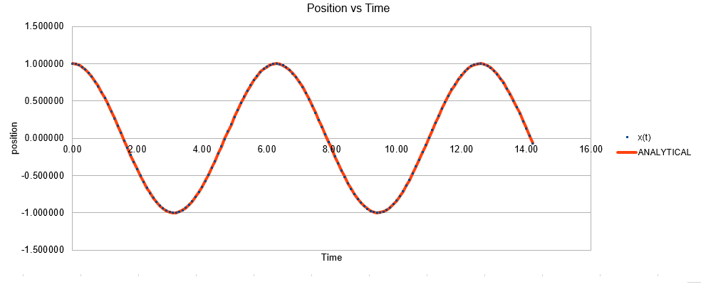
In the data given, the velocity-Verlet algorithm is used to model the behaviour of a classic harmonic oscillator. The classical position for $x$ at time $t$ was also found using the equation $x\left(t\right)=A\cos (\omega t+\varphi )$. The results for the position from both the classical and velocity-Verlet were plotted on the same axis. As can be seen, the agreement is quite good.

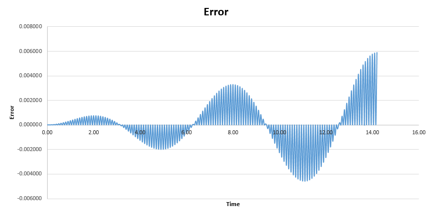
The error between this classically calculated value and the velocity-Verlet solution was also found. The graph shows how error varies with time. As the time is increased, the error gets larger, this is due to the fact that with each time step error occurs therefore as we increase the time the error of each step is summed cumulatively and so the amplitude of the graph increases.

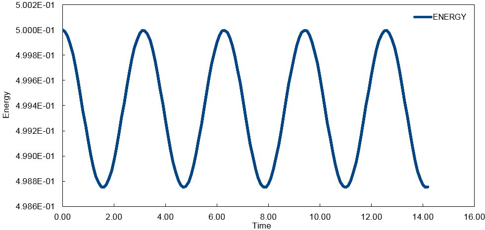
The energy was calculated using the classical formula for kinetic energy $E=\frac{1}{2}m{v}^2$ and potential energy $E=\frac{1}{2}k{x}^2$. The total energy needs to be considered when modelling it's behavior numerically in order to obtain a realistic overview of what is happening.

The smaller the time step used, the more accurately the simulation reflects reality and the smaller the change in energy over the course of the simulation. However, the time step needs to be large enough to gain a full picture of what is happening.

Leonard Jones Potential

The Lennard Jones potential is an effective way to describe the energy of an interaction between atoms in a fluid, as a function of the distance between them. It consists of a smooth attractive part at long range and steep repulsive part at short range. The simplicity and accuracy of the formula makes it ideal for use in molecular dynamic computations.

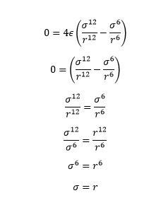
$\varphi \left(r\right)=4ϵ(\frac{{\sigma }^{12}}{r^{12}}-\frac{{\sigma }^6}{r^6})$ When the potential energy is 0, the seperation of atoms, $r_0$, is

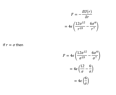
The force is equal to the negative derivative of the Lennard Jones Potential.

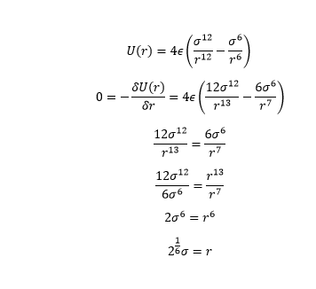
At the equilibrium bond distance, the Leonard Jones potential is at a minimum, ie. the derivative and therefore the force is 0. This is where the atom pair is most stable and will remain until it is disturbed externally.

By substituting $r(eq)$ back into the equation, the well depth was found to equal

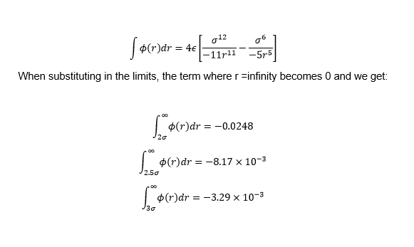
The integrals $\underset{2\sigma }{\overset{\mathrm{\infty }}{\int }}\varphi \left(r\right)\mathrm{d}r$, $\underset{2.5\sigma }{\overset{\mathrm{\infty }}{\int }}\varphi \left(r\right)\mathrm{d}r$, and $\underset{3\sigma }{\overset{\mathrm{\infty }}{\int }}\varphi \left(r\right)\mathrm{d}r$ when $\sigma =ϵ=1.0$ where evaluated.

Periodic Boundary

In 1 ml is 1g in mass. In this there are $\frac{1.0}{18}=0.055moles$

and $0.55\times 6.022\times 10^{23}=3.345\times 10^{22}atoms$

$10000$ water molecules occupies a volume of :

$\frac{18}{6.022\times 10^{23}}\times 10000=2.898\times 10^{-19}c{m}^3$

In order to carry out the simulation, the atoms are enclosed to a box of fixed dimensions. The box is repeated infinitely in all direction in order to not expose the outer atoms to vacuum. When an atoms crosses the boundary of one box, it is replicated in the next box through the opposite face as to keep the number of atoms inside the box constant.

An atom at position $(0.5,0.5,0.5)$ in a cubic simulation which runs from $(0,0,0)$ to $((1,1,1)$ moving along the vector $(0.7,0.6,0.2)$ will end up at $(0.2,0.1,0.7)$

Truncation

By introducing periodic boundary condition, other problems arise. The potential as defined earlier, is dependent on all possible pairs of atoms. If there is an infinite number of replicas of the system, we need to avoid calculating an infinite number of pair interactions.

Looking at the integrals calculated earlier for the Lennard Jones potential, we can see that attractive part dominates and and as r increases it decays quickly. From this we can assume that there is a distance beyond which interactions are so small that they can be ignored. When forces are calculated, only those where the interaction is is less that the cutoff are included.

Reduced Units

When using Lennard Jones Potentials, we often work in reduced units. In order to do this, all quantities in the simulation are divided by a scaling factor resulting in values being more managable. These reduced quantities take the form:

• distance $r^{*}=\frac{r}{\sigma }$
• energy $E^{*}=\frac{E}{ϵ}$
• temperature $T^{*}=\frac{k_{B}T}{ϵ}$

The Lennard-Jones parameters for argon are $\sigma =0.34\mathrm{n}\mathrm{m},ϵ=120/k_B\mathrm{K}$. If the LJ cutoff is $3.2$, in real units it is equal to $r=3.2\times \sigma =1.088nm$.

The well depth$=-ϵ$

$=\frac{120\times -k_B\times N_A}{1000}$ $=0.9977kJmo{l}^{-1}$

If the reduced temperature is $T^{*}=1.5$ in real units it is $180K$.

Equilibration

Five initial simulations were run in the LAMMPS software package, the melting of a crystal. In these, the time step was changed to 0.001, 0.0025, 0.0075, 0.01 and 0.015 respectively.

Creating the simulation box

In order to run the simulation, the initial states of all atoms in the system need to be specified. The amount of information needed varies depending on the type of numerical integration used. For all calculations, however, we need the starting position.

For a crystal, this information can be found by looking up the crystal structure. However, in liquids, finding the co-ordinates is more difficult due to the fact that there is no long range order.

Generating random co-ordinates for atoms in a liquid generates the desired disorder however this causes many problems; when atoms are plotted too close together the repulsion are very strong.

Instead, the atoms are placed on the lattice points of a primitive cubic lattice. Given enough time, over the simulation, the atoms are rearranged into a more realistic configuration.

In the input file; the line

lattice sc 0.8

generates a simple cubic lattice of number density 0.8. From the output file we can see the line

Lattice spacing in x,y,z = 1.07722 1.07722 1.07722

Indicating the distance between the points of the lattice is 1.07722.

This an be verified as follows. The volume of the cube is $1.07722^3=1.2500$ The density is equal to $\frac{numberofatoms}{volume}$ In a simple cubic crystal there is 1 atom, giving a density of 0.8.

If a face centred cubic lattice with a number density of 1.2 was used instead, the length of the unit cell can be calculated. There are four atoms in a FCC, therefore $volume=\frac{4}{1.2}=3.3$ $length=cbrt(3.3)=1.4938$.

The next lines in the input file define a region in space or "box", in this case extending ten lattice spacing's from the point of origin in 3 dimensions. This gives a box containing 1000 unit cells and, for the simple cubic lattice, 1000 atoms.

If we were to again consider the face centered cubic lattice, we would have 4000 atoms present.

Setting the properties of the atom

As well as the positions, we also must set the physical properties of the atoms.

mass 1 1.0
pair_style lj/cut 3.0
pair_coeff * * 1.0 1.0 

The mass command sets the mass of the atoms, the number 1 is the atom type and 1.0 is the mass. The pair_style command sets the formula LAMMPS uses to compute the pair wise interactions. Pair potentials are defined between pairs within a cutoff distance and the set of active interactions typically changes over time. lj/cut refers to the Lennard Jones cut off potential with no Coulomb.

The pair_coeff is used to specify the pair wise force field coefficient for one or more pairs of atom types.

The velocity of the atoms was also specified, ${\mathbf{x}}_i\left(0\right)$ and ${\mathbf{v}}_i\left(0\right)$, and therefore, the velocity-Verlet algorithm was used.

Running the Simulation

Instead of just writing

timestep 0.001
run 100000 

We write

### SPECIFY TIMESTEP ###
variable timestep equal 0.001
variable n_steps equal floor(100/${timestep})
variable n_steps equal floor(100/0.001)
timestep ${timestep}
timestep 0.001

### RUN SIMULATION ###
run ${n_steps}
run 100000

in the input file. This command tells LAMMPS that if it encounters the text $[timestep} on a subsequent line, it should be replaced by the value given (0.001). This is done because when comparing different timesteps we want to keep the total time of the simulation constant. By inputting the command in this way, we are able to do so; the total time will be the same, but the timestep changed.

Checking Equilibration

LAMMPS is abble to calculate a number of thermnodynamic properties, in this simulation we are interested in only the energy, temperature and pressure. These can be used to make sure the results make sense.

The data obtained from the simulations was used to plot energy, temperature and pressure against time for the 0.001 timestep.

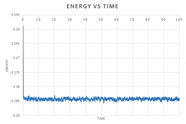
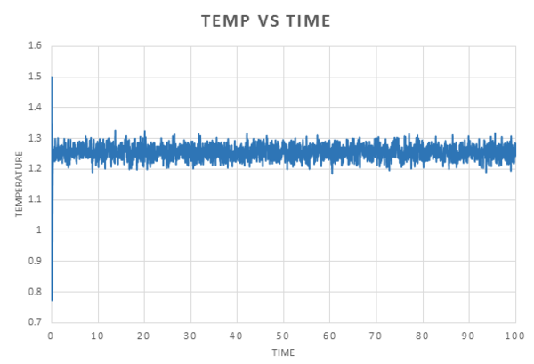
We can see from these plots that equilibrium is reached very quickly, after an initial large fluctuation, for each property, the graph converges with a small fluctuation around an average value.

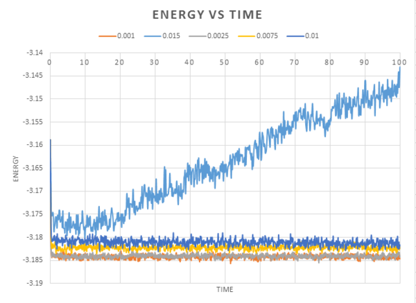
The graph below shows energy plotted against time for all of the timesteps run in this simulation, $0.001,0.0025,0.0075,0.01,0.015$.

‎

The shorter timesteps give reslts that more accurately reflect physical reality. However, if the same number of timesteps is used, the shorter timetep will cover a shorter amount of real time. Therefore a balance needs to be struck. From the graph we can see there is little difference between the accuracy when using a 0.001 time-step or 0.0025 timestep. The 0.015 timestep is particulary bad. If the simulation had worked, we would see the energy fluctuate around an average (as seen by the other timesteps), instead, the energy is rising. This disobeys the 1st law of thermodynamics, the conservation of energy.

Running simulations under specific condition

In this section, the simulation, melting of a simple cubic crystal, was changed in order to run under NpT conditions (isobaric-isothermal).

The results enabled us to plot an equation of state for our model fluid.

The pressure used was chosen by evaluating the average pressure form the previous simulation; $P=2.6,2.8$ Five temperatures were chosen above the critical temperature $T*=1.5$. $T*=1.6,2.0,3.0,4.0,5.0$.

The time step was set at 0.001. This was chosen due to the fact that the smaller the timestep, the more accurately the results reflect reality. However there is little difference between the accuracy of a 0.001 timestep and 0.0025 timestep as seen from the previous simulations. The larger timestep would mean that the simulation was run over a longer time period and so a more complete picture may be obtained. However as equilibrium is reached quickly, this is not an issue for this system.

Thermostats and Barostats

The equipartition theorem states that in equilibrium, every degree of freedom will have associated with it $\frac{1}{2}{k}_{B}T$ of energy. In our system we have N atoms, each with three degrees of freedom, hence we can write: $E_K=\frac{3}{2}N{k}_{B}T$ $\frac{1}{2}\sum _i{m}_i{v}_i^2=\frac{3}{2}N{k}_{B}T$

After each timestep, this equation is used to determine the kinetic energy and the "instantaneous" temperature $T$. $t$ tends to fluctuate around the target temperature (the value in the input script). However we can alter the temperature by multiplying the velocity by a constant, $\gamma$.

1. $\frac{1}{2}\sum _i{m}_i{v}_i^2=\frac{3}{2}N{k}_{B}T$

2. $\frac{1}{2}\sum _i{m}_i{\left(\gamma v_i\right)}^2=\frac{3}{2}N{k}_B\mathfrak{𝔗}$

These equations can be solved to find the value of $\gamma$ so that $T=\mathfrak{𝔗}$ by dividing 2 by 1. Giving

${\gamma }^2=\frac{\mathfrak{𝔗}}{T}$

$\gamma =(\frac{\mathfrak{𝔗}}{T}{)}^{\frac{1}{2}}$

Examining the input script

In the input script, we have a section dedicated to bringing the system to the required state. This allows us to keep the system at a constant temperature (it can also be used to change the temperature over the course of the simulation.

fix npt all npt temp ${T} ${T} ${tdamp} iso ${p} ${p} ${pdamp}

The section

### MEASURE SYSTEM STATE ###
thermo_style custom step etotal temp press density
variable dens equal density
variable dens2 equal density*density
variable temp equal temp
variable temp2 equal temp*temp
variable press equal press
variable press2 equal press*press
fix aves all ave/time 100 1000 100000 v_dens v_temp v_press v_dens2 v_temp2 v_press2
run 100000

is used to determine the thermodynamic properties that are recorded and measure. The line

fix aves all ave/time 100 1000 100000 v_dens v_temp v_press v_dens2 v_temp2 v_press2

is to use one or more global values as inputs every few time steps and average them over longer timescales.

The general input is

fix ID group-ID ave/time Nevery Nrepeat Nfreq value1 value2

Where Nevery (100) means use input value every this many timesteps, Nrepeat(1000) is the number of times to use input values to calculate averages and Nfreq(100000) means calculate the average over this many time steps.

Plotting the Equation of state

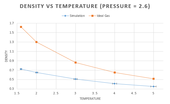
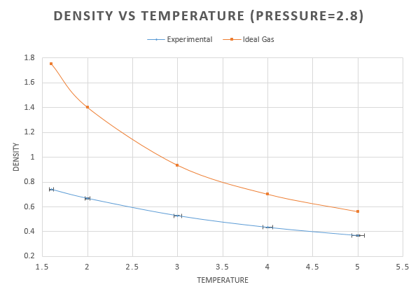
For each pressure, the density was plotted as a function of temperature along with the density calculated using the ideal gas law,$PV=nkbT$. This can be rearranged to give the density as follows: $\frac{n}{V}=\frac{P}{kbT}$. As we are working in reduced units, the boltzmann constant needs to be converted to reduced units also. This is equal to 1 and so the density becomes: $\frac{n}{V}=\frac{P}{T}$

The higher pressure shows an overall higher density. This is due to the fact that the higher pressure causes the atoms to be closer together, decreasing the volume occupied. As the density is fixed at $\frac{mass}{volume}$ decreasing the volume, therefore increases the density.

For all curves, as the temperature increases, we see a decrease in density. This is due to the fact that, with an increase in temperature comes an increase in the kinetic energy. As the atoms are moving more, more space is taken up and so the volume increases decreasing the density decreases.

At both pressures the result form the ideal gas is higher than the simulation. The ideal gas laws assumes that there are no interactions between molecules. This would allow for molecules to get closer together, reducing the volume and increasing the density. As the temperature increases, the difference between the two decreases, this is due to the fact that kinetic energy is increasing and starting to dominate how close the molecules are able to get.

Calculating heat capacities using statistical physics

Heat capacity calculation

Quantities in statistical thermodynamics can be calculated by considering how far from equilibrium the system is allowed to fluctate. For instance, when the temperature is held constant, the total energy must be fluctuating. The size of these fluctuations tells us about the heat capacity.

$C_V=\frac{\partial E}{\partial T}=\frac{\mathrm{V}\mathrm{a}\mathrm{r}\left[E\right]}{k_B{T}^2}=N^2\frac{⟨E^2⟩-{⟨E⟩}^2}{k_B{T}^2}$

The $N^2$ is required because LAMMPS divided all energy output by the number of atoms; when measuring $E$, $E/N$ is actually being measured.

The input file used for the previous section was edited in order to perform these simulations. An example of the input file is attached here.

Simulations at 10 phase points were run. Densities of $0.2$ and $0.8$ and with temperatures of $2.0,2.2,2.4,2.6,2.8$

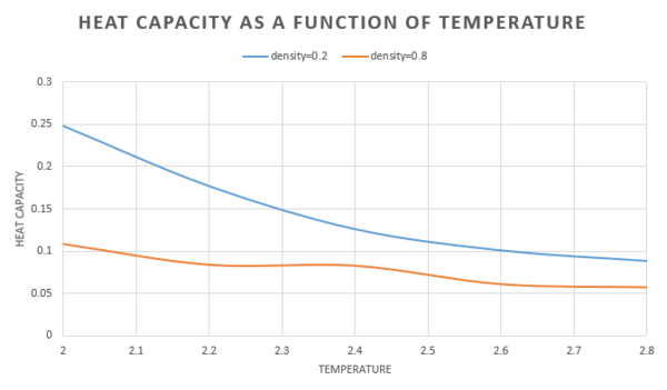
The heat capacity was the plotted as a function of temperature for both densities.

As the temperature is increased, the heat capacity decreases. This can be explained by the fact that at high temperature, the molecule is already in a high energy state, therefore it can not absorb as much energy and thus the heat capacity is lower.

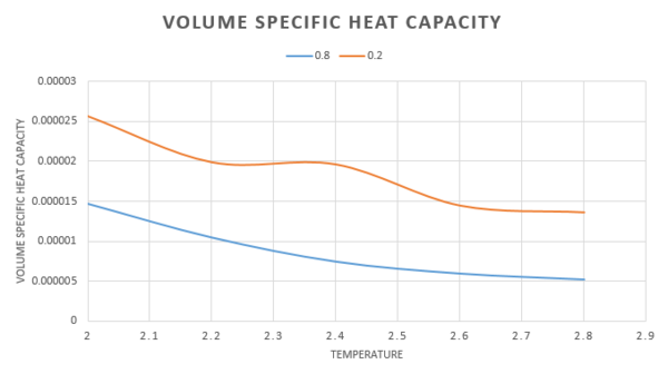
By dividing the heat capacity by the volume of the box, $4218.78$ at $density=0.2$ and $16874.92$ for $density=0.8$, we obtain a volume specific heat capacity, this is a measure of the heat capacity per unit volume, thus we are able to draw a better comparison of heat capacity at the two different densities. Now that the volume of the systems is equal, the number of atoms present will vary. As density is equal to the number of particles divided by volume, the higher density system will have a larger number of atoms present. There will be a larger number of accessible energy levels and therefore the heat capacity will also be higher. The heat capacity is an extensive property, it is proportional to the size of the system and so it follows that, it increases as we increase the number of atoms. This shown in the graph below. Again we see that as the temperature increases, the heat capacity decreases.

Structural Properties and the Radial Distribution Function

The Radial distribution function $g(r)$ is of great use in thermodyanmics, it can be used to determine many macroscopic properties of systems. It allows us to relate density with distance from a reference particle. That is, it represents the probability of finding a particle at a distance $r$ away form a reference particle. This involves determining how many particles are within $r$ and $r+\mathrm{d}r$ of the reference particle.

In this section, the Lennard Jones simulation was run three phases, solid liquid and gas, by modifying the temperature and density parameters. The values used were found from a phase diagram of the Lennard Jones system In order to simulate a solid, the parameters were changed to $T=1.0$, $\rho =1.2$. For this system a face centered cubic lattice was used. To simulate a liquid, the parameters were change to $T=1.2$, $\rho =0.8$. The gas simulation had parameters of $T=1.1$, $\rho =0.01$.

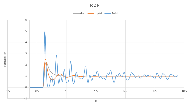
From the results obtained, VMD was used to calculate $g(R)$ and $\int g(r)\mathrm{d}r$. The graph shows math>g(r)</math> for all 3 phases.

In all phases, at very small distances, there is zero probability of finding another particle. This is due to the strong repulsions experienced at close range. The peaks observed indicate the different "shells" of neighbours, ie. the first closest neighbour, second closest neighbour etc.

In the solid RDF we can see that there are a large number of sharp peaks and these are still obvious at long range. This is indicative of the long range ordering in solid structures where the atoms are confined to a particular region in space.

The liquid RDF shows that there is some ordering at short range through the appearance of multiple peaks. However they quickly converge to 1. This is as expected for a liquid.

In the gas we see only one maximum. This is due to the fact that there is a higher degree of disorder in this phase and so the probability of finding an atom past the first nearest is very small.

At very long range all RDF's tend towards 1 as this is the average density at this range.

For the solid, the first three peaks, 1.025, 1.525 and 1.825 are the first, second and third nearest neighbours. In the face centered cubic lattice, taking a corner as the starting point, the first nearest neighbour is the atom on the adjacent face. the next nearest neighbour is situated on the next corner with the third being on the opposite face of the lattice. This is depicted in the image below:

Image source: http://www.superstrate.net/pv/physics/crystal.html

By evaluating the integral of the RDF plot we are able to determine the co-ordination number to these first three atoms. By looking at the point at which the peak ends, where it reaches a minimum, we are able to determine the co-ordination number. For the first peak, from the $g(r)$ function we can see that the peak collapses at $r=1.275$. By finding the corresponding point on the running integral, we are able to see that there are 12 atoms co-ordinated. The area under the second peak collapses at $r=1.625$ with a corresponding integral of 18. by subtracting the integral of the first peak, we find that the co-ordination of the second nearest neighbour is 6. The third peak ends at $r=1.975$ with the corresponding integral equal yo 42. Subtracting the first two peaks we obtain a co-ordination number of 24.

As demonstrated in the image above, the lattice spacing is equal to the distance between the point of origin and the second nearest neighbour. This gives a spacing of 1.525.

Dynamical Properties and the diffusion coefficient

In this section, simulations were run in order to calculate the diffusion coefficient. This is a measure of how much the atoms move around in the simulation.

Mean Squared Displacement

An easy way to measure the diffusion coefficient, $D$ is by exploiting the mean squared displacement. In statistical mechanics, this is the most common measure of spatial extent of random motion. In a molecular system a molecule does not move in a straight line; collisions with other molecules cause it to be jostled. They are equally likely to move both forward and backwards, therefore when adding the probable distance travelled, it sums up to zero. To overcome this problem, we instead add the square of each distance travelled, resulting in a positive value, the squared distance. An average over all molecules gives us the mean squared distance.

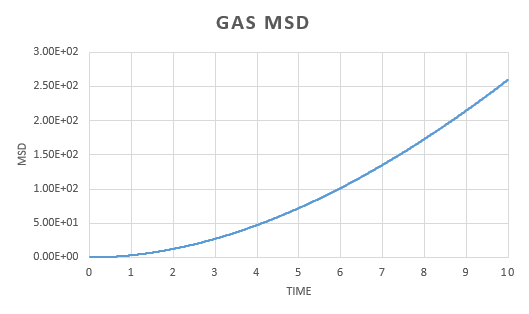
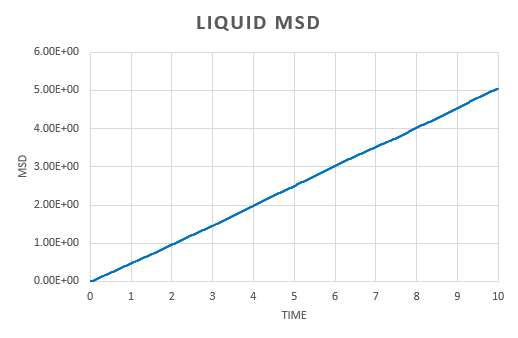
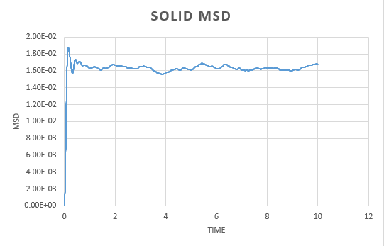
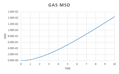
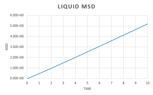
A simulation was run for a vapour, liquid and solid. Graphs were the plotted of the the total (x,y,z) mean squared displacement as a function of time step. This was then used to find $D$ using the following equation:

$D=\frac{1}{6}\frac{\partial ⟨r^2\left(t\right)⟩}{\partial t}$

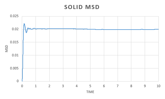
We expect to see a straight line dependence of the MSD and this is what we get in the gas and liquid phase. The gas has an initial curve, this is due to the fact that the path taken by a molecule will not resemble a straight line until a collision occurs. As the molecules in a gas are far apart, we see a curve. This is not observed in the liquid as the molecules are close together and therefore a collision occurs almost instantaneously. The graph for a solid is very different. In a solid, the atoms are held in a fixed position, this will be where the atom is most stable and it is very difficult for the atom to leave this place. Because of this highly regular, fixed structure, the area that the atom can move in is very small and what is observed is vibrations. This is reflected in the graph. We can see an initial increase before the MSD plateaus.

The plots were then used to find $D$ using the following equation:

$D=\frac{1}{6}\frac{\partial ⟨r^2\left(t\right)⟩}{\partial t}$

The slope of the graphs were found by plotting a line of best fit on the graphs and determing the gradient. By multiplying this by $\frac{1}{6}$ we were able to find D.

The diffusion constant for the gas was found to be $4.41$. As expected, this is large; the molecules are well spaced and able to move around freely and so the diffusion coefficient is large. For a liquid, the diffusion constant is lower at $0.078$ , this is due to the fact that the molecules are packed but able to move over each other in a fluid like motion. This value will vary with the viscosity of the liquid. The solid diffusion coefficient is very small $5\times 10^{-6}$. This is because the highly ordered structure of a solid allows for little diffusion to take place.

The same analysis was carried out for simulations run with one million atoms.

The plots show a similar trend to those form the simulation run earlier. The gas MSD vs time plot reaches a straight line quicker when there are one million atoms present.

The liquid plot is very similar both presenting linear dependence.

The solid plot again shows the initial increase before plateauing, however, when there are more atoms present, the fluctuations become much smaller and the plot appears smoother. As we are taking the average over a larger sample size, the effect that any fluctuations have on the appearance of the graph are reduced.

The similarities in the two sets of graphs are reflected by obtaining similar value for the diffusion coefficient; $D=2.54,0.087,5\times 10^{-6}$ for the vapor, liquid and solid respectively. Both the solid from the simulation and the one with one million atoms gives the same diffusion coefficient. There is a very small difference in liquid diffusion coefficient and the largest difference can be seen in the gas diffusion coefficient. This can be explained by the fact that when there are one million atoms present, the MSD forms a linear dependence earlier.

Velocity Autocorrelation Function

The velocity autocorrelation function is a time dependent correlation function, revealing the underlying dynamic processes in a molecular system. It essentially shows the difference in velocity of an atom between $t$ and $t+\tau$, $C\left(\tau \right)=⟨\mathbf{v}\left(t\right)\cdot \mathbf{v}(t+\tau )⟩$.

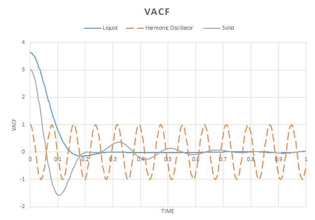
The results form the previous simulation were used to plot the VACF against time.

An atom at time zero will have a specific velocity. If this atom under goes no interactions, the atom would remain at this velocity for all time. This would result in the plot of $C(\tau )$ being horizontal.

However in solids and liquids, there are strong interatomic forces. This causes atoms to position themselves such that attractive and repulsive forces are balanced out- where that atoms are most energetically stable. In solid systems, these positions are extremely stable and atoms cannot easily move from them. The motion they possess is therefore a vibration or oscillation, with the velocity being reversed after each oscillation. This is reflected by the VACF plotted, we can see there is an oscillation between positive and negative values. However the oscillations decay over time and will eventually go to zero, reflecting a dampened harmonic oscillator. This arises because there are other, perturbative forces acting on the atom to restore it to the equilibrium position.

The VCAF plotted for the liquid shows only one minimum before decaying to zero. Liquids have similar properties to solids, however, they are able to flow due to the atoms not being in a fixed position. This fluid motion allows for the removal of an oscillation.

The minima in these graphs arise when there is a collision, resulting i n a change in velocity.

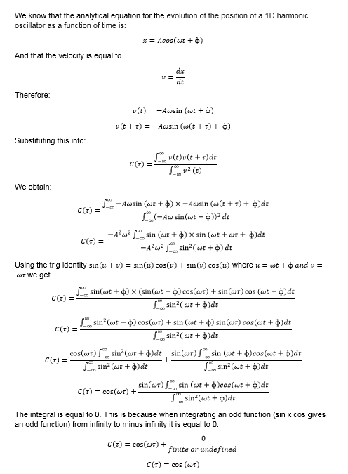
The equation for the evolution of the position of a 1D harmonic oscillator as a function of time, $x(t)=Acos(\omega t+\varphi )$ was used to evaluate the normalised velocity autocorrelation function for a 1D harmonic oscillator.

Using $\omega =\frac{1}{2\mathrm{\Pi }}$, the harmonic oscillator was also plotted on the graph resulting in a very different plot. The harmonic oscillator has a single force acting on it and so experiences no damping whilst the Lennard Jones potential has multiple forces acting on it, causing the damping effect that is observed.

The potential for a harmonic oscillator is symmetric and so the velocity has no directionalality. This is not the case for the Lennard Jones potentials. the are unsymmetrical and so we see directionality; in one direction, interactions are strongly repulsive whilst in the other they are attractive. This has an effect on the velocity and can be used to explain the damping observed.

The diffusion coefficient can also be calculated using the velocity autocorrelation function by integrating $C\left(\tau \right)=⟨\mathbf{v}\left(t\right)\cdot \mathbf{v}(t+\tau )⟩$ to give

$D=\frac{1}{3}\underset{0}{\overset{\mathrm{\infty }}{\int }}\mathrm{d}\tau ⟨\mathbf{v}\left(0\right)\cdot \mathbf{v}\left(\tau \right)⟩$.

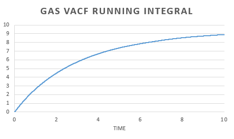
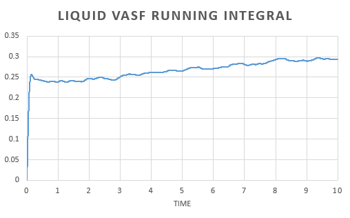
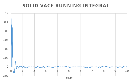
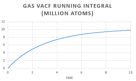
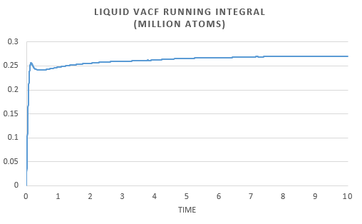
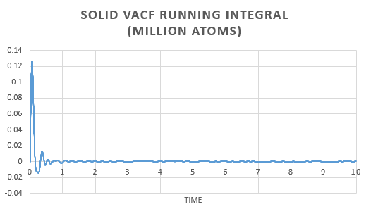
In order to estimate the integral the trapezium rule was used, $area=\frac{1}{2}h[(y_0+y_n)+2\times (y_1+y_2+...+y_{n-1})]$. Form, this we could calculate D for both the simulation and one million atom VACF. This was also used to plot a running integral.

$D=2.97$

$D=0.098$

$D=1.8\times 10^{-4}$

$D=3.27$

$D=0.090$

$D=4.5\times 10^{-5}$

The diffusion coefficient found for the simulation and the one million atom simulation are simialar. Again we can see that the gas has the largest and the solid the smallest coefficient as expected.

There is little variation in the diffusion coefficient calculated using the MSD and VACF. The variation that does arrise is due to the approximations in calculating the differential in the MSD approach and the integral in the VACF method; the trapezium rule, over or underestimates the area under the curve.

As the diffusion coefficient for a solid is so small, the variation in the result obtained is negligible.

References

- ↑ J, Meller, "Molecular Dynamics", Nature, 2001
- ↑ 2.0 2.1 2.2 http://lammps.sandia.gov/doc/fix_ave_time.html
- ↑ Jean-Pierre Hansen, Loup Verlet, "Phase Transitions of the Lennard-Jones System ", 1969. DOI:10.1103/PhysRev.184.151