Rep:Mod:P0TAT0

Molecular Dynamics Simulations of Simple Liquids

Ab9314 (talk) 11:11, 24 March 2017 (UTC)

Introduction

Molecular dynamics (MD) is a method to simulate the motion of many particles by numerically integrating Newton's Laws of Motion over time. The simulation can be conducted in an ensemble, e.g. NVT or NVE, by setting limits on temperatures and pressures (thermostatting and barostatting respectively). MD can be used to simulate the behaviour of protein folding, lipid bilayers, and other biological systems, thereby making this a very practical and convenient way to experiment with complex systems. The potential between particles were calculated using pairwise-additive 12-6 Lennard-Jones potentials. All simulations were performed on the HPC system using the LAMMPS software package.

Velocity Verlet Algorithm

To begin the simulation, a lattice of atoms can be initiated with atoms a user-defined length apart (inputted in reduced units). All particles were given an initial velocity (according to Maxwell-Boltzmann distribution). Integrating each particle's velocity over time iteratively gave the new positions of the atoms in the system. This was done using the velocity-Verlet algorithm.

At first, the timestep of the simulation was varied to observe the errors in the positions with passing time when using the velocity-Verlet algorithm. This was done by calculating the exact position of a simple harmonic oscillator, and comparing against the position given by the velocity-Verlet calculation.

For a simple harmonic oscillator, $x(t)=A\cos (\omega t+\varphi )$. Using an Excel spreadsheet, the error in the Velocity-Verlet algorithm was calculated. In this case, $A=\omega =1$ and $\varphi =0$. The error is plotted in Figure 1, and the maxima in the error is plotted against time in Figure 2.

• 
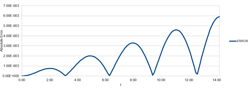  Figure 1: Error in displacement (when calculated by velocity-Verlet algorithm) against time for a simple harmonic oscillator.
• 
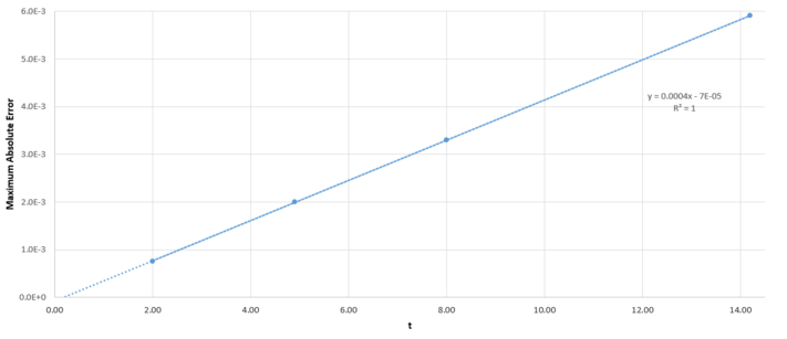  Figure 2: Maximum error in displacement against time for the harmonic oscillator.

By changing the timestep in the spreadsheet, it was found that the error in $x(t)$ as calculated by the velocity-Verlet algorithm is less than $1\mathrm{\%}$ over the course of the simulation when the timestep is less than $0.025$.

The total energy of the system should be monitored to make sure that the energy is conserved in the system, and to check if the system is in thermal equilibrium. If the total energy is not stable, then the thermodynamic values derived from the system will not be equilibrium values, and cannot be compared to other MD systems.

Atomic Forces

In order to make the calculations easier, the LJ-potentials were given a 'cut-off' distance - any atoms separated by a distance larger than this truncation distance will not be included in the LJ force calculations.

When $\sigma =ϵ=1.0$:

$\varphi \left(r\right)=4(\frac{1}{r^{12}}-\frac{1}{r^6})$

$\int \varphi \left(r\right)dr=4(-\frac{1}{12r^{11}}+\frac{1}{6r^5})+c=\frac{2}{3r^5}-\frac{1}{3r^{11}}+c$

Thus, when limits are introduced:

$\underset{2\sigma }{\overset{\mathrm{\infty }}{\int }}\varphi \left(r\right)\mathrm{d}r=-2.07\cdot 10^{-2}$

$\underset{2.5\sigma }{\overset{\mathrm{\infty }}{\int }}\varphi \left(r\right)\mathrm{d}r=-6.81\cdot 10^{-3}$

$\underset{3\sigma }{\overset{\mathrm{\infty }}{\int }}\varphi \left(r\right)\mathrm{d}r=-2.74\cdot 10^{-3}$

From the above calculations, the force of attraction reduces very quickly when the distance from the Lennard-Jones centre is greater than $2\sigma$. Hence, truncation at such a distance will introduce only a very small error in the system.

Periodic Boundary Conditions

As it is very heavy computationally to simulate even millimole amounts in LAMMPS, Periodic Boundary Conditions (PBCs) are used to cut down the calculation times. The reason for this difficulty can be seen by considering the number of particles in a small volume of water.

For example, 1 mL of water contains: $\frac{1}{18}\cdot 6.022\cdot 10^{23}=3.346\cdot 10^{22}$ molecules.

In most cases, the number of particles used will be between 10³ and 10⁴.

10⁴ water molecules take up a volume of: $\frac{10^4}{6.022\cdot 10^{23}}\cdot 18=2.99\cdot 10^{-19}mL$

PBCs allow for the relatively small number of particles in our simulation to act as though it's part of a bulk solution. To this end, the particles are simulated such that when moves off one edge of the box, it reappears on the opposite face with the same velocity. Hence, the number of particles in the box, N, is always conserved.

For example, consider an atom at $(0.5,0.5,0.5)$ in a cubic box with vertices at $(0,0,0)$ and $(1,1,1)$. If this atom moves by vector $(0.7,0.6,0.2)$ in a single timestep, then the final position of the particle will be: $(0.2,0.1,0.7)$.

Reduced Units

Reduced units are used to make the numbers more manageable.

For Argon, $\sigma =0.34nm$. Given that the LJ-cutoff in reduced units is at $r^{*}=3.2$, the cutoff in nanometers is: $r=r^{*}\sigma =3.2\cdot 0.34=1.088nm$.

Given $\frac{ϵ}{k_B}=120$,

well depth, $ϵ=120k_B=1.66\cdot 10^{-21}J=\frac{1.66\cdot 10^{-21}\cdot N_A}{1000}kJmo{l}^{-1}=9.98\cdot 10^{-1}kJmo{l}^{-1}$.

Therefore, when $T^{*}=1.5$, and given $\frac{ϵ}{k_B}=120$,

$T=\frac{ϵ}{k_B}\cdot T^{*}=120\cdot 1.5=180K$.

Equilibriation

The Simulation Box

The particles for the simulation were initiated in a simple cubic lattice structure. A random set of coordinates were not used. This was to avoid two atoms being generated too close together - this would lead to a very large potential, and cause the pair to split violently apart. This simulation would be unlikely to be a good representation of a real life scenario of a crystal melting.

In this simulation, a lattice density of 0.8 was used (0.8 lattice points per unit volume). If a face-centred cubic (fcc) lattice had been used instead, with a lattice density of 1.2, then the side length of the cubic unit cell, $a$, can be found thus:

$\rho =\frac{N}{V}$

$1.2=\frac{4\cdot 1000}{(10\cdot a{)}^3}$

$a=\frac{\sqrt[3]{\frac{4000}{1.2}}}{10}=1.49380$

Properties of atoms

The reaction conditions such as the lattice density are passed into LAMMPS using text commands in the input file. Part of the commands are shown below:

mass 1 1.0 

mass defines the property of the atom that is being defined. 1 indicates the type of particle being defined; all particles in LAMMPS are given a type, in form of an integer number. For example, if considering a mixture with 2 types of atoms, then the particles in LAMMPS would be differentiated by having type 1 and type 2 particles, and so on.

1.0 indicates the mass of the particle in g mol^-1.

pair_style lj/cut 3.0

This line defines the potential between two interacting particles. Once again, the pair_style keyword indicates the property being defined. lj/cut defines the potential as a truncated Lennard-Jones potential, while the 3.0 defines the potential to be truncated at $3.0\sigma$. Overall, the potential is being defined as:

$\varphi \left(r\right)=4ϵ[{\left(\frac{\sigma }{r}\right)}^{12}-{\left(\frac{\sigma }{r}\right)}^6]r<r_c$

pair_coeff * * 1.0 1.0

This line is defining the force that each particle exerts on all other particles is the same as that defined by the negative of the derivative of the Lennard-Jones potential.

The generated particles are then given initial coordinates, and their initial velocities. As $x_i(0)$ and $v_i(0)$ are both specified, the velocity-Verlet integration is used for the simulations.

Running the Simulation

The final lines of the input file are as follows:

variable timestep equal 0.001

variable n_steps equal floor(100/${timestep})

### RUN SIMULATION ###
run ${n_steps}

variable timestep equal 0.001 creates a variable so that any subsequent occurence of the string ${timestep} is replaced by 0.001. The number of steps the simulation is run for is also determined by the value of the timestep. By assigning a variable name to the timestep, editing the timestep value will automatically adjust the number of steps, avoiding tedious editing of the value in two different places each time the timestep is changed.

Checking Equilibriation

Several different simulations were run using different timesteps, and the total energy of the system was monitored at each step. Figure 3 shows the results of the simulations.

Figure 3: Energy vs. Time for differing timesteps

All systems reach equilibrium, except for the system where the timestep is 0.015. The equilibrium was reached by around $time\approx 0.6$ - in quite a short amount of time.

Of the five timesteps used, the largest acceptable timestep is 0.01. A particularly bad choice would be a timestep of 0.015. This is because the total energy of the system seems to be increasing indefinitely with increasing time with large fluctuations. This is a poor representation of a real system, hence this simulation timestep length is too long for this system.

NPT Simulation

This section looks at running simulation under specific conditions, using an NPT ensemble. This is done using barostats and thermostats.

Temperature and Pressure Control

Temperature, $T$, fluctuates in the simulation, and the target temperature is $\mathfrak{𝔗}$. As temperature is related to the total kinetic energy of particles within the system, the temperature is kept roughly constant by multiplying the velocities of the particles by a factor $\gamma$. Hence, these two equations can be surmised from the above, from which an expression of $\gamma$ is derived:

$\frac{1}{2}\sum _i{m}_i{v}_i^2=\frac{3}{2}N{k}_{B}T$

$\frac{1}{2}\sum _i{m}_i{\left(\gamma v_i\right)}^2=\frac{3}{2}N{k}_B\mathfrak{𝔗}⟹\frac{1}{2}{\gamma }^2\sum _i{m}_i{v}_i^2=\frac{3}{2}N{k}_B\mathfrak{𝔗}$

$\frac{1}{2}{\gamma }^2\cdot \frac{3}{2}N{k}_{B}T=\frac{3}{2}N{k}_B\mathfrak{𝔗}$

$\therefore \gamma =\sqrt{\frac{2\mathfrak{𝔗}}{T}}$

The Input Script

The thermodynamic property values of the system were periodically computed and saved to file using the following command in the input script:

fix aves all ave/time 100 1000 100000 v_dens v_temp v_press v_dens2 v_temp2 v_press2

These values are time-averaged in a specific way. The arguments 100 1000 100000 instruct LAMMPS to compute the properties every 100000 steps using preceding 1000 values in intervals of 100 values. For example, at the 200000th step, the properties are averaged using values at steps number 100100, 100200, 100300... 199000, 200000.

Plotting the Equations of State

Simulations of a crystal melting were run at two different pressures, P = 2.5 and P = 3.0, with 8 temperatures for each pressure. A graph of density against temperature was then plotted, along with the density predicted by the Ideal Gas Law with respect to temperature at these two pressures. The results are shown in Figure 4. It can be seen that in general, the MD simulation predicts a lower density than the ideal gas law. This is because the ideal gas law does not take the forces between particles into account. In the Lennard-Jones potential model, the repulsive forces are very strong (compared to the attractive forces). Hence, the MD simulations show the particles will prefer to be more spread out (i.e. less dense) so as to minimise the unfavourable repulsive forces. The discrepancy decreases with increasing temperature, because the particles in the MD systems will move further apart. This in turn decreases the magnitude of the forces between particles, bringing it closer to the ideal system of no forces between particles.

Figure 4: Density vs. Temperature for varying pressure as found by MD simulations, compared to results predicted by the Ideal Gas Law.

Heat Capacity Calculations using Statistical Physics

To investigate the effect of changing temperature on the heat capacity, a simulation was run in the NVT ensemble for two different densities ($\rho =0.2$ and $\rho =0.8$). The results of the simulations are summarised in Figure 5.

Figure 5: Heat Capacity per Unit Volume vs. Reduced Temperature for differing lattice densities.

The expected value for $\frac{C_V}{V}$ in an ideal system is:

$\frac{C_V}{V}=\frac{3}{2}\cdot N\cdot \frac{1}{V}=\frac{3}{2}\cdot \rho$

Hence, for an ideal gas, when $\rho =0.3,\frac{C_V}{V}=0.1$ and when $\rho =0.8,\frac{C_V}{V}=1.2$.

The value of $C_V$ found in the simulations are around 4 orders of magnitude smaller than what is predicted the ideal system, even at low densities (more ideal system). Also, the simulation shows variation of $C_V$ with increasing temperature (approximately $C_V\propto \frac{1}{T^n},n<2$). The value of n is unknown, and must be found by fitting different curves to the data. We know that $C_V\propto \frac{Var(E)}{T^2}$ and that $Var(E)\propto T^m,m>0$. Hence, we can estimate that $n=2-m⟹n<2$. This is in contrast to the ideal system, which predicts no variation of heat capacity with temperature.

However, qualitatively, the trends seen are reasonable. As the temperature is raised, the particles have more and more energy, yet the number of available degrees of freedom fall. As $C_V$ is a measure of how easily the system is excited to higher energy states - an already excited system requires even more energy to put the particles in a higher vibrational energy states. Increasing the number of particles, $N$, also leads to a larger number of degrees of freedom, leading to an increase in the heat capacity, $C_V$. Consequently, increasing $\rho =\frac{N}{V}$ also leads to an increase in $\frac{C_V}{V}$. This trend is clearly seen in Figure 3.

Finally, the apparent reversal in trends from $T^{*}=2.3$ to $T^{*}=2.4$ is showing the change from a liquid to a gaseous phase.

The Input Script

One of the scripts used for running the NVT simulations is shown below:

### CREATING VARIABLE TO DEFINE LATTICE DENSITY
variable rho equal 0.8

### DEFINE SIMULATION BOX GEOMETRY ###
lattice sc ${rho}
region box block 0 15 0 15 0 15
create_box 1 box
create_atoms 1 box

### DEFINE PHYSICAL PROPERTIES OF ATOMS ###
mass 1 1.0
pair_style lj/cut/opt 3.0
pair_coeff 1 1 1.0 1.0
neighbor 2.0 bin

### SPECIFY THE REQUIRED THERMODYNAMIC STATE ###
variable T equal 2.2
variable timestep equal 0.0025

### ASSIGN ATOMIC VELOCITIES ###
velocity all create ${T} 12345 dist gaussian rot yes mom yes

### SPECIFY ENSEMBLE ###
timestep ${timestep}
fix nve all nve

### THERMODYNAMIC OUTPUT CONTROL ###
thermo_style custom time etotal temp press
thermo 10

### RECORD TRAJECTORY ###
dump traj all custom 1000 output-1 id x y z

### SPECIFY TIMESTEP ###

### RUN SIMULATION TO MELT CRYSTAL ###
run 10000
unfix nve
reset_timestep 0

### BRING SYSTEM TO REQUIRED STATE ###
variable tdamp equal ${timestep}*100
variable pdamp equal ${timestep}*1000
fix nvt all nvt temp ${T} ${T} ${tdamp}
run 10000
reset_timestep 0

### ENDING NVT ONCE SYSTEM IN REQUIRED STATE. NVE RESTATED.
unfix nvt
fix nve all nve

### MEASURE SYSTEM STATE ###
thermo_style custom step etotal temp press density
variable temp equal temp
variable temp2 equal temp*temp
variable eng equal etotal
variable eng2 equal etotal*etotal
fix aves all ave/time 100 1000 100000 v_temp v_temp2 v_eng v_eng2
run 100000

variable avetemp equal f_aves[2]
variable errtemp equal sqrt(f_aves[5]-f_aves[2]*f_aves[2])

### CALCULATION OF C_V
variable vareng equal (f_aves[8]-f_aves[7]*f_aves[7])
variable cv equal (3375*3375*${vareng})/(${avetemp}*${avetemp})

### PRINTING CALCULATED VALUES TO OUTPUT FILE
print "Averages"
print "--------"
print "Temperature: ${avetemp}"
print "Stderr: ${errtemp}"
print "Heat Capacity: ${cv}"

Structural Properties and the Radial Distribution Function

The Radial Distribution Function (RDF, or $g(r)$) can provide some insight into the structure of the particles in the simulation. The three phases, solid, liquid and gas, have distinctive RDF plots. These RDF plots can be compared directly to X-Ray diffraction plots produced experimentally, so that the identity of the systems can be verified by this property. Figure 6 shows the RDF plots acquired by varying the density and temperature of the NVT simulation.

• 
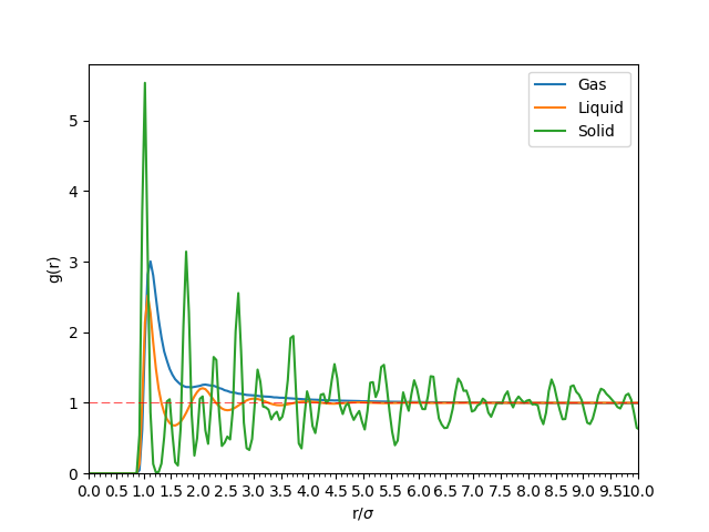  Figure 6: The RDF of the same particles in solid, liquid and gaseous phase. The initial part of the graph where $RDF=0$ indicates space between adjacent particles. This figure also shows that $g(r)$ tends to $1$ as $r$ becomes large.
• 
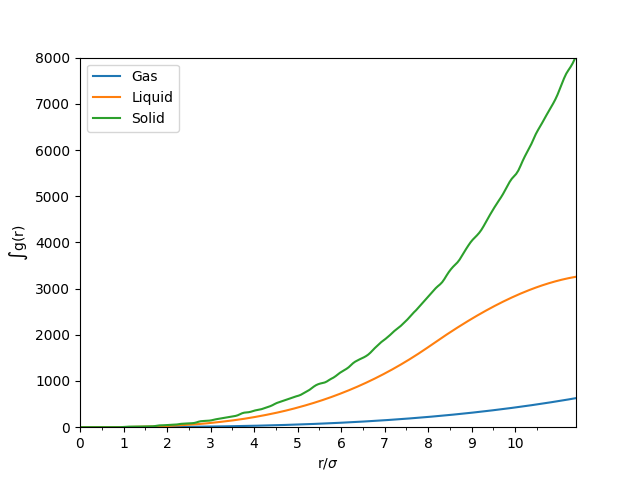  Figure 7: The integral of the RDF of the same particles in solid, liquid and gaseous phase.

Figure 8: Three closest neighbours of each atom on an face-centred lattice shown by vectors 1, 2 and 3 in increasing order of magnitude.

As can be seen from Figure 6, from $\sigma =0$ to $\sigma \approx 1$ is where the repulsive forces between the adjacent atoms are too great to be overcome, and hence is empty space.

The RDF of solids have sharp peaks at well defined spacing. The atoms responsible for each of the first three main peaks are outlined in Table 1 using Figure 8 as a reference. The lattice parameter is the distance between two adjacent atoms on the fcc lattice along a straight edge (i.e. not diagonally adjacent). This appears to be approximately $1.775\sigma$. The RDF decreases slowly as the radius increases.

By using the plot of $\int g(r)\mathrm{d}V$ against $r$ (see Figure 7), the coordination number around a single reference atom as the distance, $r$, increases. The coordination numbers at symmetry related lattice vectors 1, 2 and 3 for this fcc lattice are tabulated in Table 1.

Table 1: Summary of data inferred from RDF data.

Vector	Distance from central atom/$\sigma$	Coordination Number
1	1.025	8
2	1.775	8
3	2.725	16

The liquid has a smooth RDF, with the peaks similar distances apart, but its decay is faster than that of the solid's. The progressively smaller peaks indicate the coordination shells around each atom.

Finally, the RDF of the gas phase tends to 1 very quickly, with no visible oscillations about $g(r)=1$. This indicates a uniform distribution of particles in the simulation box, as is expected of a gas in equilibrium.

Dynamical properties and the Diffusion Coefficient

Mean Square Displacement (MSD)

Figure 9: A particle moving from initial position r(0) at time $0$ to another position r(t) at time $t$.

The motion of the particles in the molecular simulation were investigated by finding several properties of the systems.

The Mean Square Deviation (MSD) of the system is a measure of how freely the particles in the system can move to a new position (see Figure 9). The MSD is calculated thus:

$MSD=[\mathbf{r}\mathbf{(}\mathbf{0}\mathbf{)}-\mathbf{r}\mathbf{(}\mathbf{t}\mathbf{)}{]}^2$

Hence, as time progresses in a system with diffusion, the sum of MSD over all time intervals will be increasing. As $t\to \mathrm{\infty }$, the rate of increase of MSD is approximately constant. The diffusion coefficient, $D$, is defined as:

$D=\frac{1}{6}\frac{\partial ⟨{\mathbf{r}}^2\mathbf{(}\mathbf{t}\mathbf{)}⟩}{\partial t}$

This equation is true as $t\to \mathrm{\infty }$; at small values of $t$, there are few or no collisions, and the increase in $MSD\propto t^2$. $D$ can thus be estimated by fitting a straight line to the linear portion of a plot of $MSD$ against time. Figures 10, 11, 12 and 13 show the calculation of the diffusion coefficient from the $MSD$ plots. Table 2 records the values of $D$ - a clear trend of increasing values of diffusion coefficients with decreasing density can be seen from the data. Atoms in gases can therefore diffuse 20 times as fast as atoms in solids.

• 
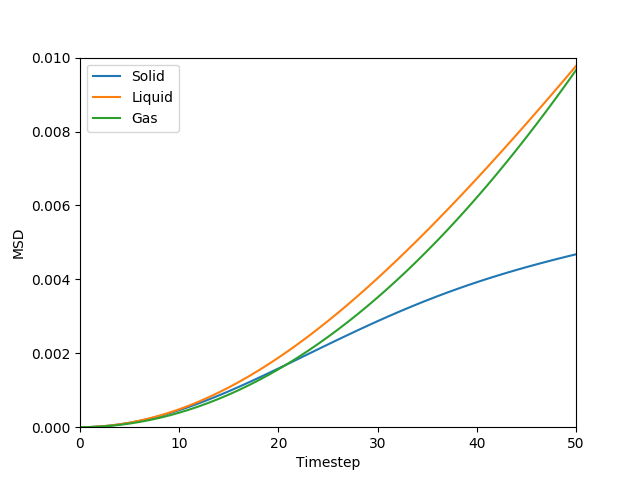  Figure 10: The MSD of the particles at at all states. The values increases with relation to time - the fastest increase is for the gas phase, followed by the liquid phase, and the solid phase is the slowest.
• 
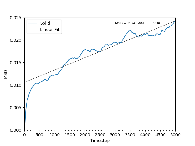  Figure 11: The MSD of the particles in the solid phase. As the particles' movements are restricted and not averaged, the plot is not smooth.
• 
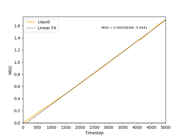  Figure 12: The MSD of the particles in the liquid phase. The plot is linear, indicating $MSD\propto t$.
• 
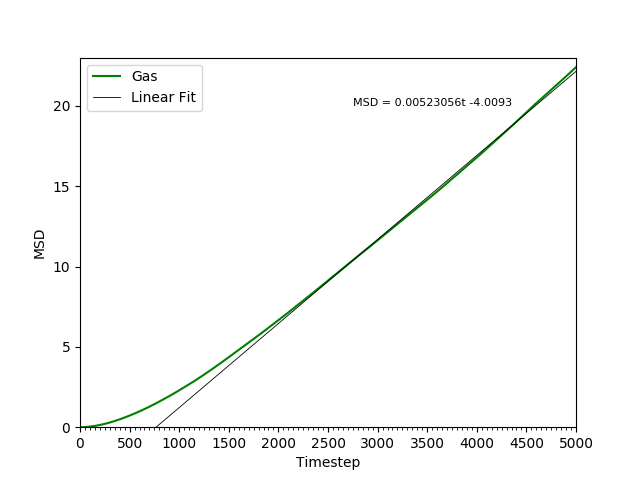  Figure 13: The MSD of the particles in the gas phase. Initially, $MSD\propto t^2$, but as $t\to \inf ,MSD\propto t$.

Table 2: Diffusion coefficient data for solid, liquid and gaseous states.

State	${\rho }^{*}$	Diffusion Coefficients, $D/{\sigma }^{2}timeste{p}^{-1}$
Solid	1.3	$2.74\cdot 10^{-6}$
Liquid	0.8	$3.47\cdot 10^{-4}$
Gas	0.1	$5.23\cdot 10^{-3}$

The above simulations were performed with thousands of particles, and this can be considered as a relatively small amount - not even a fraction of a femtomole of atoms. To simulate a larger system, a set of simulations were run with 1 million atoms. The difference in the MSD plots (see Figures 14, 15, 16 and 17) is most marked in the solid state - whereas in the smaller system, there was a definite increase in MSD over time for all timesteps, the larger system oscillates slowly oscillates around $MSD=0.0066$. Physically, this observation shows that most of the particles in the solid are vibrating and colliding into each other very often. In the smaller system, the collisions are much less frequent, so that $|\mathbf{r}\mathbf{(}\mathbf{0}\mathbf{)}-\mathbf{r}\mathbf{(}\mathbf{t}\mathbf{)}|$ is larger for each atom. The diffusion coefficients of the million atoms in the three states are tabulated in Table 3.

• 
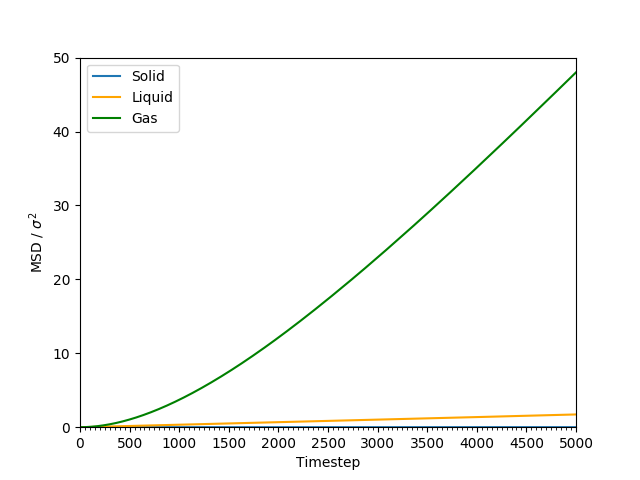  Figure 14: The MSD of the 1 million particles at at all states.
• 
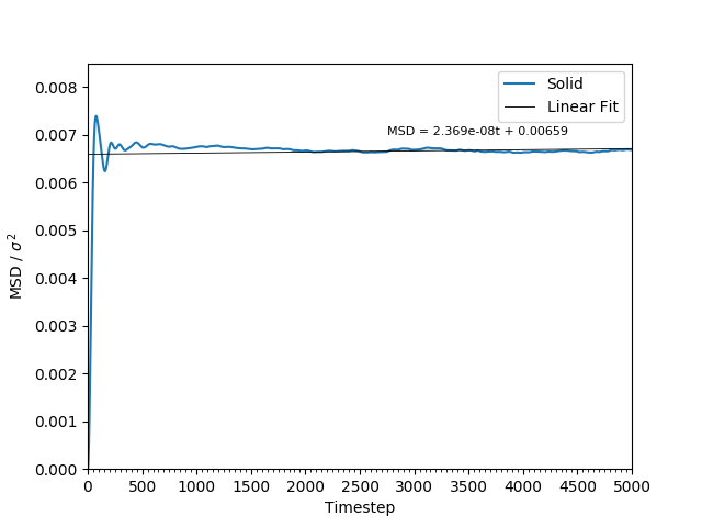  Figure 15: The MSD of the particles in the solid phase. This plot is jagged, and the gradient is almost $0$: indicating virtually no diffusion in solid state.
• 
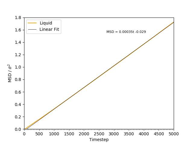  Figure 16: The MSD of the particles in the liquid phase. The plot is linear from $t=1000$.
• 
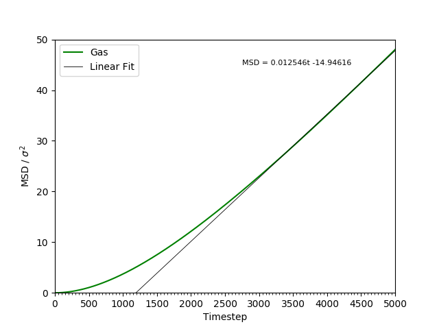  Figure 17: The MSD of the particles in the gaseous phase. The plot is linear from $t=3000$.

Table 3: Diffusion coefficient data for 1 million atoms in solid, liquid and vapour states.

State	Diffusion Coefficients, $D/{\sigma }^{2}timeste{p}^{-1}$
Solid	$2.37\cdot 10^{-8}$
Liquid	$3.50\cdot 10^{-4}$
Gas	$1.25\cdot 10^{-2}$

Velocity Autocorrelation Function

The diffusion coefficient, $D$, can also be estimated from the velocity autocorrelation function (VACF), $C(\tau )$, if $C(\tau )\to 0$ at large $\tau$:

$C(\tau )=⟨\mathbf{v}\mathbf{(}\mathbf{t}\mathbf{)}\cdot \mathbf{v}\mathbf{(}\mathbf{t}\mathbf{+}\mathit{\tau }\mathbf{)}⟩$

$D=\frac{1}{3}\underset{0}{\overset{\mathrm{\infty }}{\int }}⟨\mathbf{v}\mathbf{(}\mathbf{0}\mathbf{)}\cdot \mathbf{v}\mathbf{(}\mathit{\tau }\mathbf{)}⟩\mathrm{d}\tau$

Below, the normalised velocity autocorrelation function is evaluated for a 1D harmonic oscillator.

Given $C(\tau )=\frac{\underset{-\mathrm{\infty }}{\overset{\mathrm{\infty }}{\int }}v\left(t\right)v(t+\tau )\mathrm{d}t}{\underset{-\mathrm{\infty }}{\overset{\mathrm{\infty }}{\int }}{v}^2(t)\mathrm{d}t}$, and $x(t)=A\cos (\omega t+\varphi )⟹v(t)=-A\omega \sin (\omega t+\varphi )$:

$C(\tau )=\frac{\underset{-\mathrm{\infty }}{\overset{\mathrm{\infty }}{\int }}A\omega \sin (\omega t+\varphi )A\omega \sin [\omega (t+\tau )+\varphi )]\mathrm{d}t}{\underset{-\mathrm{\infty }}{\overset{\mathrm{\infty }}{\int }}{A}^2{\omega }^2{\sin }^2(\omega t+\varphi )\mathrm{d}t}$

Simplifying,

$C(\tau )=\frac{\underset{-\mathrm{\infty }}{\overset{\mathrm{\infty }}{\int }}\sin (\omega t+\varphi )\sin [\omega (t+\tau )+\varphi )]\mathrm{d}t}{\underset{-\mathrm{\infty }}{\overset{\mathrm{\infty }}{\int }}{\sin }^2(\omega t+\varphi )\mathrm{d}t}$

Using the trigonometric identity $\sin (a+b)\equiv \sin (a)\cos (b)+\sin (b)\cos (a)$, the following can be surmised:

$\sin [\omega (t+\tau )+\varphi )]=\sin (\omega t+\omega \tau +\varphi )=\sin (\omega t+\varphi )\cos (\omega \tau )+\cos (\omega t+\varphi )\sin (\omega \tau )$

Hence,

$C(\tau )=\frac{\underset{-\mathrm{\infty }}{\overset{\mathrm{\infty }}{\int }}{\sin }^2(\omega t+\varphi )\cos (\omega \tau )+\sin (\omega t+\varphi )\cos (\omega t+\varphi )\sin (\omega \tau )\mathrm{d}t}{\underset{-\mathrm{\infty }}{\overset{\mathrm{\infty }}{\int }}{\sin }^2(\omega t+\varphi )\mathrm{d}t}$

$C(\tau )=\frac{\cos (\omega \tau )\underset{-\mathrm{\infty }}{\overset{\mathrm{\infty }}{\int }}{\sin }^{}(\omega t+\varphi )+\sin (\omega \tau )\underset{-\mathrm{\infty }}{\overset{\mathrm{\infty }}{\int }}\sin (\omega t+\varphi )\cos (\omega t+\varphi )\mathrm{d}t}{\underset{-\mathrm{\infty }}{\overset{\mathrm{\infty }}{\int }}{\sin }^2(\omega t+\varphi )\mathrm{d}t}$

Rearranging ${\sin }^2(x)\equiv \frac{1-\cos (2x)}{2}$,

$C(\tau )=\cos (\omega \tau )+\frac{\sin (\omega \tau )\underset{-\mathrm{\infty }}{\overset{\mathrm{\infty }}{\int }}\sin [2(\omega t+\varphi )]\mathrm{d}t}{2\underset{-\mathrm{\infty }}{\overset{\mathrm{\infty }}{\int }}\frac{1-\cos [2(\omega t+\varphi )]}{2}\mathrm{d}t}$

Simplifying,

$C(\tau )=\cos (\omega \tau )+\frac{\sin (\omega \tau )\underset{-\mathrm{\infty }}{\overset{\mathrm{\infty }}{\int }}\sin [2(\omega t+\varphi )]\mathrm{d}t}{\underset{-\mathrm{\infty }}{\overset{\mathrm{\infty }}{\int }}1-\cos [2(\omega t+\varphi )]\mathrm{d}t}$

$C(\tau )=\cos (\omega \tau )+\frac{\sin (\omega \tau )\cdot \frac{1}{2\omega }[\cos (\mathrm{\infty })-\cos (-\mathrm{\infty })]}{\underset{-\mathrm{\infty }}{\overset{\mathrm{\infty }}{\int }}1-\cos [2(\omega t+\varphi )]\mathrm{d}t}$

However, $\cos (-a)=\cos (a)$ as this is an even function.

Thus, $\cos (\mathrm{\infty })-\cos (-\mathrm{\infty })=0$:

$\therefore C(\tau )=\cos (\omega \tau )$

This result shows that for a simple harmonic oscillator, the VACF is a sinusoidal function that depends on the time passed, as well as the frequency of the oscillator.

The VACF of the solid and liquid states were calculated during the simulations. In addition, the analytical solution to the VACF of a particle doing simple harmonic motion with frequency, $\omega =\frac{1}{2\pi }$ was also calculated. These are all plotted in Figure 18.

• 
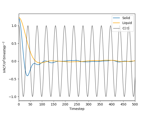  Figure 18: The plots of velocity autocorrelation functions with for atoms in a solid, a liquid, and for a simple harmonic oscillator. At large $t$, $C(\tau )\to 0$ for the solid and liquid systems.
• 
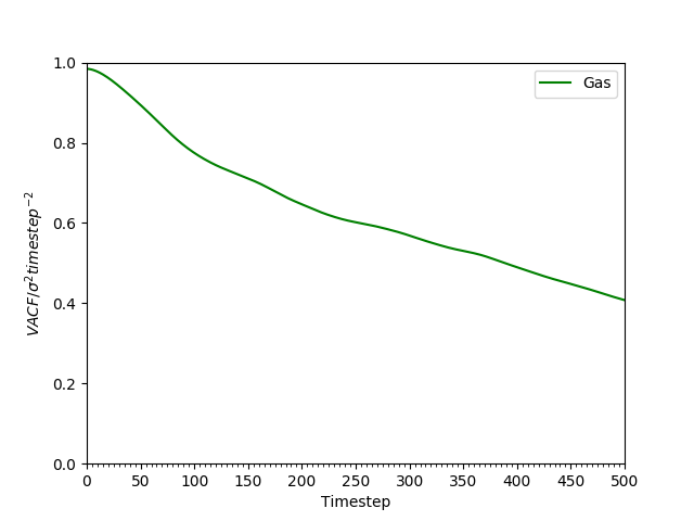  Figure 19: VACF of atoms in the gaseous phase decay much more slowly owing to the much weaker interatomic forces.

From Figure 18, it can be observed that the VACF of the simple harmonic oscillator is sinusoidal, whereas the liquid and solid VACF are best described as damped sinusoidal. The solid's VACF tends to 0 faster that that of the liquid.

The global minima in the plots for the solid and liquid indicate when all the particles have had at least one collision. By this point, each of the atoms have a different velocity vector associated with it. Hence, the VACF rebounds towards 0. As the simple harmonic oscillator is a lone particle's motion, with no interactions with any other atoms, hence its VACF is very different to the Lennard-Jones solid and liquid. Its velocity vector also changes in a cyclic manner, and does not change from one oscillation to another. Hence, the amplitude of the VACF does not change as time increases.

In the solid, the particles are in close contact due to the high density - the atoms are arranged so that the repulsive forces are minimised, and the attractive forces maximised. This is the distance at which the LJ-potential is at a minimum. Here, the atoms are very stable, and are reluctant to leave the locations they are at.Their motion is therefore a vibration around their eqiulibrium positions, with a reversal of velocity at the end of each oscillation. This explains the oscillatory behaviour of the VACF. However, the damping is explained by perturbative forces acting on the atoms that disrupt the oscillations. Liquids are similar to solids - however, the density here is lower, and diffusion is faster. Here, the diffusive forces are the perturbative forces, and hence the VACF decays much more rapidly than the solid's VACF.

In contrast, the VACF from a system in the gaseous state (see Figure 19) decays much more slowly. The large separation distances between particles in the gaseous phase mean the forces are weaker. Hence, the inter=particle forces between them only affect their velocities very slowly, over a long time. For this reason, the VACF decays much more slowly than the liquid and the solid VACF.

• 
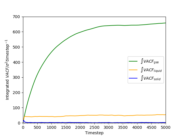  Figure 20: Cumulative integral of VACF against time for all phases as an approximation to the diffusion coefficient.
• 
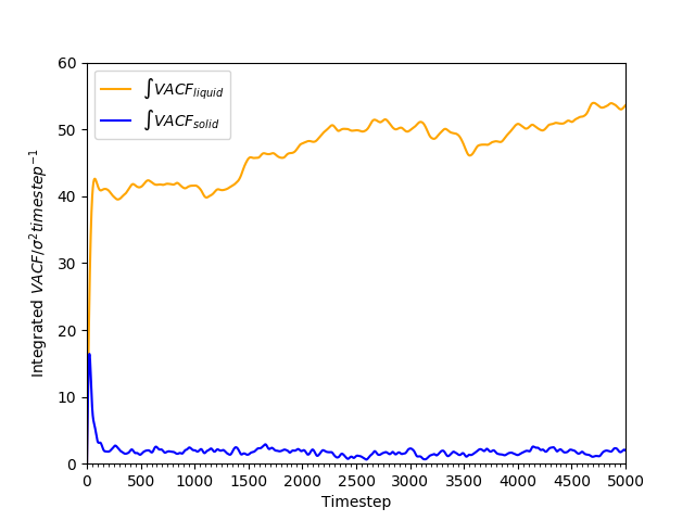  Figure 21: Cumulative integral of VACF against time for solid and liquid phases.

The area under the VACF, and thus the diffusion coefficient, $D$, was estimated by using the trapezium rule, by using the following formula:

$D=\frac{1}{3}\underset{0}{\overset{\mathrm{\infty }}{\int }}⟨\mathbf{v}\mathbf{(}\mathbf{0}\mathbf{)}\cdot \mathbf{v}\mathbf{(}\mathit{\tau }\mathbf{)}⟩\mathrm{d}\tau$

The cumulative integral is plotted in Figures 18 and 19. The gas has a very large $D$, compared to the liquid and the solid; the diffusion coefficient of the liquid is approximately 100 times as large as that of the solid. The trend of lower $D$ with higher density is as found earlier in Tables 2 and 3.

• 
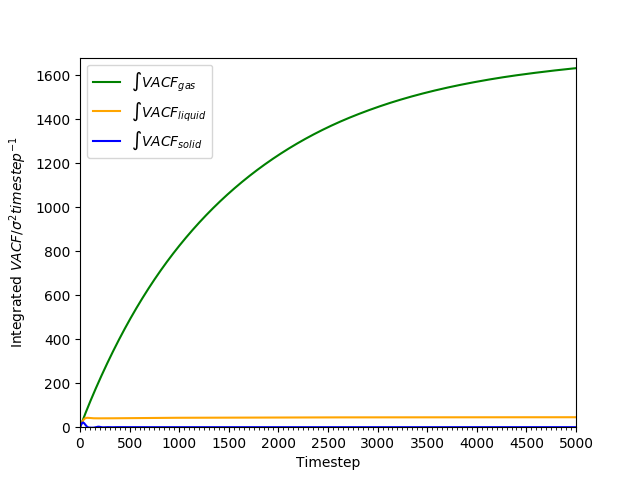  Figure 22: Cumulative integral of VACF against time for all phases for 1 million atoms.
• 
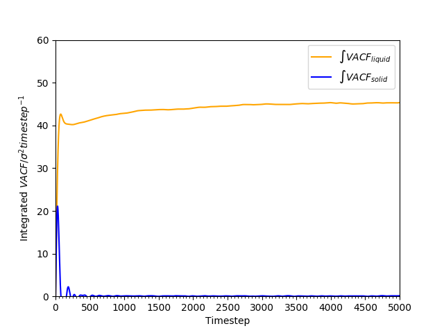  Figure 23: Cumulative integral of VACF against time for solid and liquid phases for 1 million atoms.

Table 4: Diffusion coefficient data derived from MSD and VACD compared for solid, liquid and gaseous states.

State	Diffusion Coefficients (MSD), $D/{\sigma }^{2}timeste{p}^{-1}$	Diffusion Coefficients (VACD), $D/{\sigma }^{2}timeste{p}^{-1}$
Solid	$2.37\cdot 10^{-8}$	$0.0487$
Liquid	$3.50\cdot 10^{-4}$	$15.1$
Gas	$1.25\cdot 10^{-2}$	$544$

A larger system with a million atoms was also simulated to simulate a system more akin to a real-life system. These plots (see Figures 22 and 23) are much smoother and give a more accurate value of the diffusion coefficient, $D$. The values of $D$ acquired for the 1 million atom simulation from the VACD is compared to that of the values acquired from the MSD in Table 4. The table shows $D$ values gotten from the VACD values are much higher than those derived from the MSD values. The largest source of errors of calculation of $D$ from VACF is from the use of trapezium rule to approximate the area under the graph.

References

- ↑ Godehard Suttman, "Classical Molecular Dynamics", NIC Series, 2002, 10, 211-254.>
- ↑ Karplus, Martin, "Molecular dynamics simulations of biomolecules", Nature Structural Biology, 2002, 9, 646-652, DOI: 10.1038/nsb0902-646.
- ↑ 3.0 3.1 3.2 3.3 Allen, M.P., Tildesley, D.J., "Computer Simulation of Liquids", Oxford: Clarenden Press, 1987, 1, 27-29. Cite error: Invalid
<ref>tag; name "RDF" defined multiple times with different content - ↑ Dinsdale, A.T., "SGTE data for pure elements", CALPHAD, 1991, 15(4), 317-425.