Rep:Mod:NMA1509

Part 2: Introduction to Molecular Dynamics:

- TASK: Open the file HO.xls. In it, the velocity-Verlet algorithm is used to model the behavior of a classical harmonic oscillator. Complete the three columns "ANALYTICAL", "ERROR", and "ENERGY": "ANALYTICAL" should contain the value of the classical solution for the position at time t, "ERROR" should contain the absolute difference between "ANALYTICAL" and the velocity-Verlet solution (i.e. ERROR should always be positive -- make sure you leave the half step rows blank!), and "ENERGY" should contain the total energy of the oscillator for the velocity-Verlet solution.

See figures 1, 2 & 3. The total energy in figure 3 is calculated by adding kinetic and potential energy as follows: $E_{t o t} = 0.5 * m * v^{2} + 0.5 * k * x^{2}$

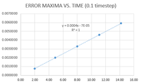
- TASK: For the default timestep value, 0.1, estimate the positions of the maxima in the ERROR column as a function of time. Make a plot showing these values as a function of time, and fit an appropriate function to the data.

See figure 4. This shows that the error in the calculation of the position increases with time. This is because it is cumulative: we use the position at time t to estimate the position at time t+timestep, so the error keeps adding up.

- TASK: Experiment with different values of the timestep. What sort of a timestep do you need to use to ensure that the total energy does not change by more than 1% over the course of your "simulation"? Why do you think it is important to monitor the total energy of a physical system when modelling its behavior numerically?

The total energy must be monitored to make sure that the principle of conservation of energy is conserved. Looking at figure 3, the energy reaches a maximum value of 0.5; 1% of 0.5 is 0.005 so to keep the energy within 1% of 0.5, it must oscillate between 0.495 and 0.500. By gradually increasing the timestep in the excel sheet provided, we find that the largest timestep that keeps the energy above 0.495 is 0.2.

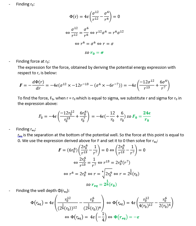
- TASK: For a single Lennard-Jones interaction, find the separation, r(0), at which the potential energy is zero. What is the force at this separation? Find the equilibrium separation, r(eq), and work out the well depth (phi). Evaluate the integrals when sigma = epsilon = 1.

- TASK: Estimate the number of water molecules in 1ml of water under standard conditions. Estimate the volume of 10000 water molecules under standard conditions.

Water has a density ρ = 1 g/mL and the molecular weight of water is 18.02 g/mol so 1 g of water has 1/18.02= 0.055 mol of water. Hence, the number of molecules that corresponds to is $0.055 * 6.022 * 1 0^{23} = 3.3 * 1 0^{22}$ molecules. As for the volume of 10000 molecules of water, that is obtained as follows: 10000 molecules are equal to $10000 / (6.022 * 1 0^{23} = 1.661 * 1 0^{- 20} m o l$ . This corresponds to a mass of $1.661 * 1 0^{- 20} * 18.02 = 2.992 * 1 0^{- 19} g$ . Knowing that the density of water is 1 g/mL, the volume is obtained by dividing mass by density which gives $V = 2.992 * 1 0^{- 19} m L$

- TASK: Consider an atom at position (0.5, 0.5, 0.5) in a cubic simulation box which runs from (0,0,0) to (1,1,1). In a single timestep, it moves along the vector (0.7, 0.6, 0.2). At what point does it end up, after the periodic boundary conditions have been applied?.

Adding up the coordinates of the atom and those of the translation vector, we can get the coordinates of the atom at the end of its movement, which are (1.2, 1.1, 0.7). Now, knowing that after crossing the boundary (1, 1, 1), the atom 're-enters' the lattice from the other side, we subtract the coordinates of the boundary from those calculated above, so the atom ends up at the point of coordinates (0.2, 0.1, 0.7).

- TASK: The Lennard-Jones parameters for argon are sigma = 0.34 nm, epsilon/k_B= 120 K. If the LJ cutoff is r^* = 3.2, what is it in real units? What is the well depth in {kJ/mol}? What is the reduced temperature T^* = 1.5 in real units?

$r^{*} = r / σ = 3.2$ and $σ = 0.34 n m$ so $r = r^{*} * σ = 3.2 * 0.34 = 1.088 n m$ ;

$ϵ = 120 * 1.38 * 1 0^{- 23} = 1.66 * 1 0^{- 21} J$ which in kJ is $1.66 * 1 0^{- 24} k J$ and multiplying by Avogadro's number gives $0.997 k J . m o l^{- 1}$ ;

$T^{*} = k_{B} T / ϵ = 1.5$ so $T = 1.5 * 120 = 180 K$

Part 3: Equilibration:

- TASK: Why do you think giving atoms random starting coordinates causes problems in simulations?

Two atoms can be generated unrealistically close to each other, yielding very high potential energy values.

- TASK: Satisfy yourself that this lattice spacing corresponds to a number density of lattice points of 0.8. Consider instead a face-centred cubic lattice with a lattice point number density of 1.2. What is the side length of the cubic unit cell?

If the lattice spacing is $1.07722$ then the volume is $V = 1.0772 2^{3}$ . So knowing that the number of lattice points is 1 in a simple cubic unit cell, then the number density is $1 / 1.0772 2^{3} = 0.8$ . As for a face centered cubic lattice, there are 4 lattice points per unit cell so if the number density is 1.2 then the volume is $4 / 1.2 = 3.3$ so the side length is 1.5.

- TASK: Consider again the face-centred cubic lattice from the previous task. How many atoms would be created by the create_atoms command if you had defined that lattice instead?

1000 atoms are created for 1000 unit cells for a cubic lattice (which has one atom per unit cell). If a Face Centered Cubic lattice is used instead, there are 3 extra atoms (or lattice points) per unit cell. So for 1000 unit cells, 3000 extra atoms would be created when changing the lattice type, giving a total of 4000 atoms (1000+3000).

- TASK: Using the LAMMPS manual, find the purpose of the following commands in the input script:

Mass command: 'mass 1' specifies that it's the value of the mass of type 1 atoms that is being considered. The value of the mass is then set (in this case, it's 1.0).

The overall command is: mass 1 1.0

pair_style lj/cut command: this computes the standard 12/6 Lennard-Jones potential to simulate the pairwise interactions between the molecules in the system; they are called 'pairwise' because the interactions considered are not limited to two specific atoms or molecules; it can be between any two and they can change, because the interaction doesn't involve a bond. This type of interaction is specified by the use of the command 'pair'; 'style' is followed by the type of pairwise interaction being considered, which is the Lennard-Jones potential; 'cut' indicates the cutoff distance (the distance from which we consider the interaction is too small to be considered and so we ignore it).
pair_coeff * * 1.0 1.0: this specifies the coefficient for the pairwise interaction between any two pairs of atoms. The asterisk takes into account any atom from 1 to N (where N is the number of atom types). There are two asterisks because we are considering a pairwise interaction involving two atoms so we must specify that we are considering all atom types for each atom in a pair. Then the value of the coefficient is given (1.0). Both coefficients are the same because the interaction is symmetric.

- TASK: Given that we are specifying position AND velocity at t(0), which integration algorithm are we going to use?

We will use the Velocity-Verlet algorithm

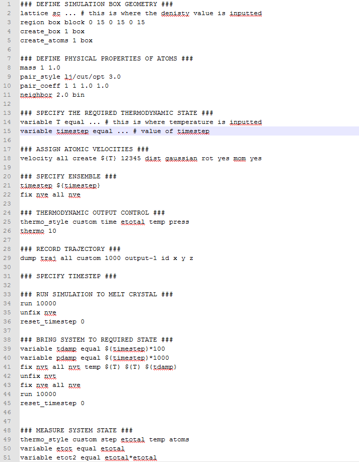
- TASK: The second line (starting "variable timestep...") tells LAMMPS that if it encounters the text ${timestep} on a subsequent line, it should replace it by the value given. In this case, the value ${timestep} is always replaced by 0.001. In light of this, what do you think the purpose of these lines is? Because we want to be able to change the timestep easily. If we only write timestep 0.001, then we would have to go through the whole script and change the values of the timestep manually everywhere it appears (including the values of the parameters that depend on the timestep, such as the number of steps). So by having these lines, if we want to change the timestep, we only need to change the value in the second line that starts with variable timestep, and it will be changed automatically throughout the script.

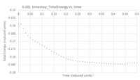
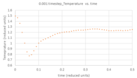
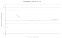
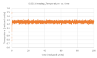
- TASK: make plots of the energy, temperature, and pressure, against time for the 0.001 timestep experiment (attach a picture to your report). Does the simulation reach equilibrium? How long does this take? When you have done this, make a single plot which shows the energy versus time for all of the timesteps (again, attach a picture to your report). Choosing a timestep is a balancing act: the shorter the timestep, the more accurately the results of your simulation will reflect the physical reality; short timesteps, however, mean that the same number of simulation steps cover a shorter amount of actual time, and this is very unhelpful if the process you want to study requires observation over a long time. Of the five timesteps that you used, which is the largest to give acceptable results? Which one of the five is a particularly bad choice? Why?

Figures 5 - 7 are plots of total energy, temperature and pressure against time. Figures 8 - 10 are the same but only look at the time between 0 and 0.5 reduced units to determine the point at which the system reaches equilibrium. For the 0.001 timestep, the system does reach equilibrium. Looking at the region between t=0 and t=0.5, equilibrium is reached at t≈0.3. Looking at Figure 11, the largest timestep to give acceptable results is 0.0025 because the fluctuations for this timestep are very small (almost the same as the 0.001 timestep) and it gives a very similar result to the smallest timestep as well. However, the smaller 0.001 timestep involves more simulations than the 0.0025 timestep for a given amount of time; if the system is studied over 1 second, the former timestep involves 1000 simulations whereas the latter only involves 400. The largest timestep, 0.0015, is a very bad choice as the total energy deviates significantly from the average value starting from ~ 20 time reduced units. This is because the larger the timestep, the larger the error associated with each energy value for the velocity-verlet solution, and these errors keep accumulating. This is illustrated by the Error in position vs time graph attached above.

Part 4: Running simulations under specific conditions:

- TASK: We need to choose $γ$ so that the temperature is correct $T = τ$ if we multiply every velocity by $γ$ . Find an expression for $γ$ .

- TASK: Use the manual page to find out the importance of the three numbers 100 1000 100000. How often will values of the temperature, etc., be sampled for the average? How many measurements contribute to the average? Looking to the following line, how much time will you simulate?

Every 100 timesteps, values of the temperature, pressure, energy and density will be sampled. 1000 measurements will contribute to the average, which will be calculated after 100 000 timesteps (i.e. simulation will last 100 000 timesteps).

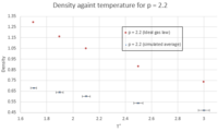
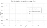
- TASK: When your simulations have finished, download the log files as before. At the end of the log file, LAMMPS will output the values and errors for the pressure, temperature, and density. Use software of your choice to plot the density as a function of temperature for both of the pressures that you simulated. Your graph(s) should include error bars in both the x and y directions. You should also include a line corresponding to the density predicted by the ideal gas law at that pressure. Is your simulated density lower or higher? Justify this. Does the discrepancy increase or decrease with pressure?

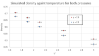
For the ideal gas law, the values for the density were obtained as follows: $N / V = p / k_{B} T$ Figures 12 and 13 show that in both cases (p = 2.2 and p = 2.6), the simulated density is lower than that obtained from the ideal gas law. This is because the ideal gas law assumes that the potential energy in the system is only due to thermal energy; i.e. it ignores interatomic interactions. In reality, these do have an effect on the density, as shown by the outcome of the simulations. The density will be lower in a real situation compared to an ideal gas because of the repulsive interaction between atoms, which prevents having the same number of atoms as an ideal gas in a specific volume. However, as we go to higher temperatures, the simulated value and the value from the ideal gas law are closer (smaller discrepancy). That's because when T is very high, the thermal energy factor, which confers to the atoms their kinetic energy, overrides the interatomic repulsion: when kinetic energy is very high, atoms move around very quickly so if we're focusing on a specific volume, we'll find that the number of atoms in that volume decreases with increasing temperature. Hence the simulated density value and the density value from the ideal gas law are more similar. As for the general trend observed in figures 12 - 14, as expected, density decreases with increasing temperature because increasing temperature implies higher kinetic energy associated with each atom, so they repel each other more strongly, thus reducing the number of atoms present in a given volume.

Part 5: Calculating Heat Capacity using Statistical Physics:

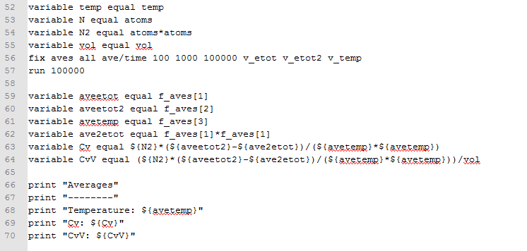
- TASK: As in the last section, you need to run simulations at ten phase points. In this section, we will be in density-temperature phase space, rather than pressure-temperature phase space. The two densities required at 0.2 and 0.8, and the temperature range is 2.0, 2.2, 2.4, 2.6, 2.8. Plot C(v)/V as a function of temperature, where V is the volume of the simulation cell, for both of your densities (on the same graph). Is the trend the one you would expect? Attach an example of one of your input scripts to your report.

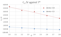
See figure 15. Comparing the two curves at different densities, at a higher density, the heat capacity is generally higher (across all temperatures) because higher density means more atoms (or molecules) per unit volume, which means more energy will have to be put into the system to reach a certain temperature, given that there are more molecules that need to be raised to higher energy levels to bring the system to that higher temperature.

As for the trend for the variation of $C_{v} / V$ against temperature for one specific density, it can be seen that $C_{v} / V$ decreases as the temperature increases. A possible explanation behind this is that, as the temperature of the system increases, the energy levels are more closely spaced. So, if a system is at a high temperature, less energy will be required to raise its temperature by one degree compared to a situation in which the system is at a lower temperature, where energy levels are further apart, and so where more energy has to be put into the system to raise its temperature by one degree.

Finally, comparing the slopes of the two curves, the slope of the curve at higher density is larger than the slope at a lower density. A possible reason behind this is that at a higher density, there are more molecules per unit volume, so there is a higher probability of finding the molecules at a higher energy level when heat is transferred to the system, so less energy has to be put into the system to raise its temperature by one degree and take the system into a level higher in energy than the previous one, simply because more molecules are at a high energy level initially. Whereas in a less dense system, there are overall less molecules per unit volume so the probability of finding many of these molecules at a high energy level is lower, so more energy has to be put in so that the molecules that are in an energy level below the average are brought up to the same excited level as the other molecules, which started off at a higher energy anyway.

Note: the script is inserted below

Part 6: Structural properties and the Radial Distribution Function:

-TASK: perform simulations of the Lennard-Jones system in the three phases. When each is complete, download the trajectory and calculate g(r) and the integral of g(r)dr. Plot the RDFs for the three systems on the same axes, and attach a copy to your report. Discuss qualitatively the differences between the three RDFs, and what this tells you about the structure of the system in each phase. In the solid case, illustrate which lattice sites the first three peaks correspond to. What is the lattice spacing? What is the coordination number for each of the first three peaks?

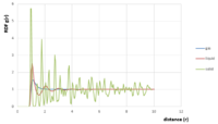
See figure 16. The Radial distribution function g(r) is the ratio between the value of the density in a shell of a given volume at a distance r from a reference atom and the density of the whole system. As such, when g(r) = 1, that means the density in that specific shell is the same as the overall density. So starting from the centre of the atoms (or molecule) that is the reference and moving away from that centre along a straight line, the RDF remains equal to 0 as long as the distance r by which we have moved is lower than the radius of the atom (or molecule). When r is greater than that radius, there is high probability that many neighbouring atoms (or molecules) will be found at that radius, around the atom, and given that we are still close to the reference atom, the volume of the shell at distance r is small and so the density in that shell (number of atoms/ volume) will be larger than the overall density, thus making g(r)>1.

Overall, looking at figure 16, as r increases, g(r) fluctuates between values greater than and smaller than 1 (in the latter case, the ‘local’ density in the shell being considered is lower than the overall density). At large r, g(r) goes to 1; i.e. when we are far enough from the reference atom, the ‘local’ density is the same as the bulk, or overall, density.

These fluctuations mentioned earlier differ depending on the phase of the system. Looking at the RDF for the gas phase, g(r) goes to 1 rather quickly and that is representative of the fact that atoms or molecules in the gas phase are very far apart so after that first peak, the probability of finding neighbours decreases very quickly. For a liquid, g(r) takes longer to stabilise at 1 simply because the atoms/ molecules are closer together and there is more ‘order’ in a liquid.

Finally, for the solid which is the most closely packed and ordered structure, we must get to a much higher distance r before the number of atoms/molecules in the shell being considered is the same as the overall density. So, as long as r is small when looking at a solid, the amount of atoms/molecules in that sphere will represent a higher density than the overall one.

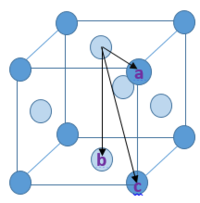
A FCC lattice is shown in diagram 1. It shows the nearest three lattice sites to the atom that is chosen as a reference (i.e. the one in the centre of the top face). The distance from the reference to atom b is equal to a (the lattice parameter); using Pythagoras Theorem, the distances reference to atom a and reference to atom c are found to be $a * 2^{0.5} / 2$ and $a * (3 / 2)^{0.5}$ respectively. These three lattice sites correspond to the first three peaks in the RDF. To find a, we can look at figure 16 and read the r value at which occurs the second peak. This is found to be $a = 1.475$ .

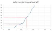
The above mentioned ‘local’ density is obtained by dividing the number of atoms found in the shell being considered by the volume of that shell. The number of atoms in that shell is called ‘coordination number’. The coordination number for a shell at a distance r be obtained by looking at the curve for the number integral over g(r) (Figure 17 - obtained from VMD calculations) and looking at where the curve reaches a plateau: the r value towards the beginning of the plateau is the lattice site and the g(r) value at the end of the plateau (before g(r) begins to increase again) is the coordination number. The number integral over g(r) is, however, cumulative. So if the number integral at the first lattice point is 12 and at the second it's 18, then the coordination number at the first lattice point is 12 and at the second it is $18 - 12 = 6$ . The number integral at the third lattice point is 42. The coordination number is then $42 - 18 = 24$ . The reason we do not do 42-18-12 is that the second number integral (18) already takes into account the first one, so by doing 42-18-12, we would be subtracting double the number of atoms which are in the first shell.

Part 7: Dynamical properties and the diffusion coefficient:

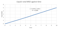
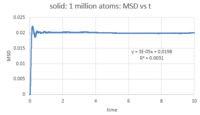
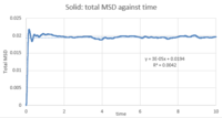
- TASK: make a plot for each of your simulations (solid, liquid, and gas), showing the mean squared displacement (the "total" MSD) as a function of timestep. Are these as you would expect? Estimate D in each case. Be careful with the units! Repeat this procedure for the MSD data that you were given from the one million atom simulations.

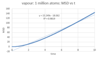
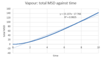
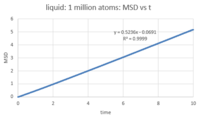
The number of timesteps was converted to time by multiplying it by the timestep (0.002). After plotting MSD against time (figures 18 - 20), the diffusion coefficient was calculated by multiplying the slop of the linear fit by 1/6. The diffusion coefficient for each phase is:

Vapour: D = 2.5228
Liquid: D = 0.0846
Solid: D = 0.000005

This behavior is expected: atoms move around freely in the vapour phase; in the liquid phase, there is more order and the atoms are closer together (higher density) so there is less 'free' space around each atom for it to move around; as for the solid, atoms are closely packed and their positions are 'fixed' (they are not completely static, however). Since D is characteristic of how much the atoms move in the phase in question, it will be highest for the vapour phase, lower for the liquid phase and ~ 0 for the solid phase. Looking at the MSD curve for the solid, there is initially a sharp increase before the total MSD fluctuates around a fixed value (~ 0.02). This is probably because as soon as we start the simulation for the solid, the atoms are assigned random velocities so they move around randomly for a short period before interatomic interactions regulate their movement. This is, however, very quick and of very small magnitude, comparing with the liquid and vapour phases where total MSD reaches 5 and 160 reduced units respectively. Note that the command responsible for assigning random velocities is velocity all create ${temperature} 12345 dist gaussian rot yes mom yes.

Repeating the same procedure for a system containing 1 million atoms (figures 21 - 23), the following results were obtained for D:

Vapour (1 million atoms): D = 2.5415
Liquid (1 million atoms): D = 0.087267
Solid (1 million atoms): D = 0.000005

The values are almost the same as those previously found for the much smaller system. This shows that D is a property of the atom, rather than the whole system. As such, it does not depend on the size of the system (intensive property).

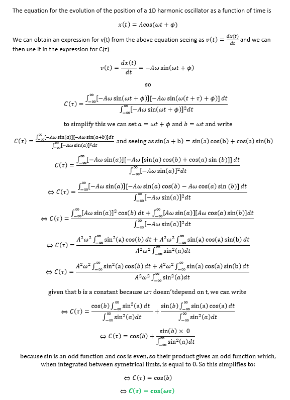
- TASK: In the theoretical section at the beginning, the equation for the evolution of the position of a 1D harmonic oscillator as a function of time was given. Using this, evaluate the normalised velocity autocorrelation function for a 1D harmonic oscillator (it is analytic!). Be sure to show your working in your writeup. On the same graph, with x range 0 to 500, plot $C (τ)$ with omega = 1/2*pi and the VACFs from your liquid and solid simulations. What do the minima in the VACFs for the liquid and solid system represent? Discuss the origin of the differences between the liquid and solid VACFs. The harmonic oscillator VACF is very different to the Lennard Jones solid and liquid. Why is this? Attach a copy of your plot to your writeup.

Working for normalised velocity autocorrelation function for a 1D harmonic oscillator:

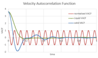
Figure 24:Normalised VACF and VACF of L-J solid and liquid

To understand the shape of the curves shown in Figure 24, we consider an atom that has a given initial velocity and position. If the atom does not interact with anything around it, it would retain the values of those initial conditions. However, that is not what happens in reality, given that the atom interacts with other atoms surrounding it. If the atom has some free space to move in (i.e. not a very dense system), it will vibrate and move around its initial position, while interacting with atoms around it (repulsive and attractive interactions). All this will affect the value of its initial velocity in both magnitude and direction. That is why the VACF goes to zero: because after a certain point in time, the value of the velocity is no longer correlated to the initial value. In a solid, more dense, system, it will take longer for the VACF to stabalise at 0 because the atoms are less free to move around and the interactions they have with neighboring atoms do not change much over time because everything is closely packed so the values of the velocity remain correlated for longer. Hence in the VACF of the solid, the curve oscillates a bit, as the direction of the velocity vector changes, and the magnitude 'slowly' goes to 0 (it at least goes to 0 slower than in the liquid system). As for the minima in the liquid and solid VACFs, these correspond to collisions between atoms, which then move away from each other. The reason these collisions occur at the beginning of the simulation (even for a well packed solid) is because of the random velocity that is assigned to each atom at the beginning of the simulation. The command that is responsible for this is:

velocity all create ${temperature} 12345 dist gaussian rot yes mom yes

Despite the fact that the distribution of these random velocities follows the Maxwell-Boltzmann distribution, it still means that it is very likely that 2 atoms next to each other will be assigned a velocity that leads to a collision because each velocity vector is pointing directly towards the other atom.

As for the harmonic oscillator, its VACF continues to oscillate around 0 with the same magnitude. This is because it ignores the fact that beyond a certain interatomic distance r, the attractive forces will be too weak to keep the two atoms in question near one another; on the other hand, below a certain distance r', the repulsive forces are too great and the atoms will, in reality, want to move away from each other. It assumes that they will maintain the same interaction until infinity, which is why the VACF shows that the correlation between velocity values over time will not eventually go to 0.

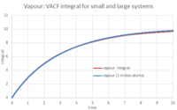
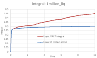
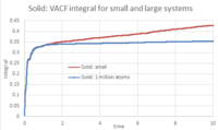
- TASK: Use the trapezium rule to approximate the integral under the velocity autocorrelation function for the solid, liquid, and gas, and use these values to estimate D in each case. You should make a plot of the running integral in each case. Are they as you expect? Repeat this procedure for the VACF data that you were given from the one million atom simulations. What do you think is the largest source of error in your estimates of D from the VACF?

The integral was calculated according to the trapezium rule, then plotted against time. To calculate D, the value of the integral at t = 10 was multiplied by 1/3. The density values are recorded below:

For the small system:

- Vapour: D = 3.224

- Liquid: D = 0.152

- Solid: D = 0.143

For the 1 million atoms system:

- Vapour: D = 3.268

- Liquid: D = 0.101

- Solid: D = 0.118

The plots of the running integrals are as expected. Figures 25 - 27 show the running integrals for the 3 phases in both the small and large systems. In the case of the solid and liquid systems, there is a rapid increase in the running integrals at the beginning. This is due to the large peak present in the VACF plots (see figure 24). The Integral then quickly stabalises because the VACF goes to ~0. As for the vapour phase, there is no sharp peak in the running integral because in the VACF of a gas, the curve does not dip to a minima at the beginning, like in the case of a solid or liquid. These values deviate strongly from those calculated previously. The largest source of error in calculating D from the VACF is the way the integral of the VACF is calculated: we approximate the area underneath the curve to a series of trapeziums where the height h is equal to the timestep, and where the two bases of the trapezium are equal to the values of the VACF at t and at t + timestep. Note that seeing as the VACF oscillates and goes below 0, the absolute value of VACF is used when estimating the integral.