
Rep:Mod:La409Mod3
Laurence Archer - Computational chemistry laboratory Module 3
Introduction
The aim of this investigation is to use molecular modelling and computational calculations to interrogate 'the transition state' of chemical reactions. Two straightforward case studies which have a simple transition state are the Cope rearrangement and Diels-Alder reaction, where the transition states consist of a six-membered ring (adopting either the chair or boat conformers). The reactant molecule in the Cope rearrangement however is highly conformationally flexible and so initially the conformers are investigated so as to ascertain the most favourable structure. The two transition states are then investigated using two different methods, with the differences and similarities being highlighted. Finally, the Diels-Alder reaction is investigated by: the reactant molecule Molecular Orbitals being analysed, transition state geometry computed and regioselectivity studied.
The Cope Rearrangement


Introduction
The Cope Rearrangement is a [3,3]-sigmatropic rearrangement of 1,5-dienes. It was discovered in 1940 by Arthur Cope, who at the time was investigating introduction of substituted vinyl groups into (dialkylvinyl)-cyanoacetates.[1] Cope found that when he formed ethyl (1-methylpropenyl) allylcyanoacetate, as per Scheme 1, the compound was unstable and formed a product of higher boiling point after several distillations; this only occurred when the allyl halide was used in Step 2, increasing the chain length resulted in stable products that did not undergo this rearrangement. Cope deduced that 1,5-dienes can undergo a pericyclic rearrangement if it results in a more stable product; this rearrangement was later named the 'Cope rearrangement'.[2]
The aim of this section is to model 1,5-hexadiene along the reaction coordinate of its Cope rearrangement, shown in Scheme 2. This will involve exploring the various conformers the reactant can adopt, modelling the transition state using a number of different methods, and visualising the product of the reaction after the transition state decomposes. For the purpose of this investigation the Hartree-Fock calculation method is used with a 3-21G basis set as this low-level method suffices in accurately modelling this system.
The Reactant
The reactant molecule 1,5-hexadiene is highly conformationally flexible due to free rotation about the central carbon-carbon bond and relative orientation of the terminal vinyl groups, hence all possible conformers were first modelled in Gaussview and optimised using the HF/3-21G method in Gaussian.
A list of all obtained conformers is shown below. In these images, the highlighted blue atoms refer to C-H bonds that the plane of the neighbouring vinyl groups align with.
| Name | Structure | Point group | Energy / Hartrees | Relative energy / kcal/mol |
|---|---|---|---|---|
| Anti 1 |  |
C2 | -231.6926 | 0.04 |
| Anti 2 |  |
C2h | -231.6854 | 4.6 |
| Anti 3 |  |
Ci | -231.6925 | 0.1 |
| Anti 4 |  |
C1 | -231.6910 | 1.0 |
| Gauche 1 |  |
C2 | -231.6877 | 3.1 |
| Gauche 2 |  |
C2 | -231.6917 | 0.6 |
| Gauche 3 |  |
C1 | -231.6927 | 0.0 |
| Gauche 4 |  |
C2 | -231.6915 | 0.7 |
| Gauche 5 |  |
C1 | -231.6896 | 1.9 |
| Gauche 6 |  |
C1 | -231.6892 | 2.2 |

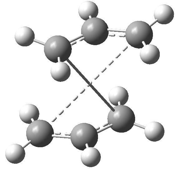
Here it can be seen that the Gauche 3 rotamer is the lowest in energy. Based purely on steric interaction one would expect the anti forms to have a lower energy, but the HOMO of the Gauche 3 form is stabilised by an interaction between the two π-bonds, as can be seen by the picture on the right.
The Anti 3 form was then optimised using the B3LYP/6-31G DFT method and the geometry of the final products compared. A summary of the main measurements of the geometry is shown below.
| Parameter | HF | B3LYP |
|---|---|---|
| Dihedral 1 | 120.0 | 120.0 |
| Dihedral 2 | 114.7 | 118.5 |
| Angle 1 | 119.7 | 119.0 |
| Angle 2 | 124.8 | 125.3 |
| Angle 3 | 112.7 | 112.7 |
| Length (C=C) | 1.32 | 1.33 |
| Length (C-C) | 1.51 | 1.50 |
Note: 'Dihedral 1' represents the dihedral around the central C-C bond. 'Dihedral 2' represents the dihedral around the allyl C-C single bond. 'Angle 1' represents the angle between the C=C bond and the vinyl hydrogen on what can be considered carbon 2. 'Angle 2' represents the angle in the allyl carbon framework. 'Angle 3' represents the angle between the central C-C bond and its neighbouring C-C bond.
As can be seen there is a small difference in these values, with the most notable difference being in 'Dihedral 2'.
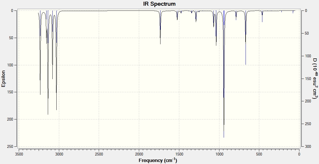
Frequency analysis
The vibrational output showed only real frequencies, with the smallest values being 74.7 cm-1, 79.2 cm-1 and 122.0 cm-1. IR spectrum
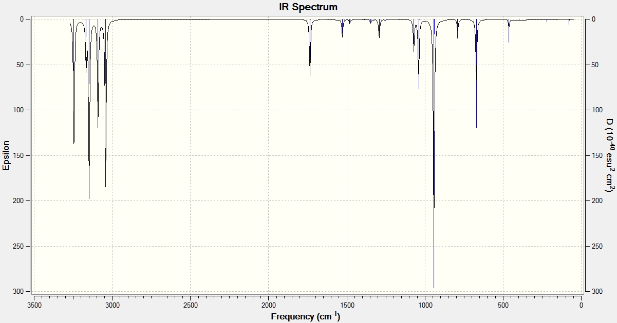
The frequency analysis was then repeated at 0K. The vibrational output showed only real frequencies, with the smallest values being 74.8 cm-1, 79.3 cm-1 and 122.2 cm-1. IR spectrum
Thermochemistry
| Energy | 298 Kelvin | 0 Kelvin |
|---|---|---|
| Electronic + Zero Point Energies | -234.469 | -234.469 |
| Electronic + Thermal Energy | -234.492 | -234.461 |
| Electronic + Thermal Enthalpy | -234.461 | -234.460 |
| Electronic + Thermal Free Energies | -234.501 | -234.500 |
It can be noted that the 'Electronic + Zero Point Energies' do not change at 0 Kelvin, due to the fact that the zero point energy in this value represents the energy of the system at' 0 K.
The Transition State
Due to the conformational flexibility of the reactant, the six-membered ring transition state to the Cope rearrangement can exist in the chair or boat conformers. This section will use differing methods to model both these transitions structures.
Chair optimisation
By looking back at Scheme 2, it can be seen that the chair transition structure can be visualised as two allyl fragments positioned anti to one another with two transitions bonds connecting them. Thence to begin with an allyl fragment was optimised by HF/3-21G (resulting structure Energy: -115.82 Hartrees, RMS Gradient Final: 0.000029, Dipole: 0.0292 Db, Point group: C2v) and the resulting structure duplicated into the same Molecular Group in Gaussview, positioned ~2.2 Å apart.
Optimising to a Transition State (Berny)

|
| [3] |
The first optimisation was performed using the following parameters:
# opt=(calcfc,ts,noeigen) freq hf/3-21g geom=connectivity |
This job performed an optimisation to a transition state (not to a local minimum) by using the Berny algorithm, paired with a frequency analysis of the optimised structure. Here we compute an approximated Hessian matrix of force constants at the first optimisation iteration by invoking the 'calcfc' keyword. This determines the direction of negative curvature on the potential energy surface at the 'guess' transition structure of, thus determining the reaction coordinate. The keyword 'NoEigen' is also invoked so as to prevent the optimisation calculation crashing if more than one imaginary frequency is detected.
The resulting structure of this optimisation is shown on the right. It can be seen that the distance between the two allyl fragments has lowered from the guessed 2.20 Å to 2.02 Å, indicating this to be the optimum distance as a transition state according to the Berny algorithm. The vibrational analysis showed the presence of a large negative frequency at -818 cm-1, this being an imaginary frequency. When a molecule exists at a minimum on its potential energy surface, any vibration in the structure involves moving up the potential energy surface away from equilibrium, having a positive force constant (derived from the second derivative of the potential energy). When at a transition state however, any vibration along the axis of the reaction coordinate will have a negative force constant, because the vibration lowers the molecule down the potential energy surface. Under simple harmonic motion approximations, the frequency of this vibration is proportional to the square root of the force constant, hence when the force constant is negative the frequency will be an imaginary number. This imaginary frequency vibrational mode of -818 cm-1 is shown in the link on the right, as expected bearing a vibration along the reaction coordinate axis.
The disadvantage of this method is that calculations are performed over the whole of the structure and so any significant inaccuracies in the 'guess' transitions structure can affect the computed direction of the reaction coordinate. The next method used resolves this problem by in effect specifying the known reaction coordinate, thus only calculating force constants along the required coordinate.
Optimising using redundant coordinates
This method first involves using the Redundant Coordinate Editor in Gaussview to 'freeze' the coordinates of the atoms that make up the 'transition bonds' that form and break simultaneously at a pre-set value determined to be close to the ideal length, in this case: 2.20 Å. Optimisation to a stable minimum is then performed on the rest of molecule to 'clean it up' as such using the following method parameters:
# opt=modredundant hf/3-21g geom=connectivity
...
B 11 3 2.200000 F
B 14 6 2.200000 F
The frozen coordinates are then relieved and instead the two transition bonds are now labelled to have their second derivatives along this coordinate calculated while undergoing the Berny optimisation to a transition state method. In this way, the transition state optimisation only calculates force constants along the specified coordinate. The used parameters were:
# opt=(ts,modredundant,noeigen) freq rhf/3-21g geom=connectivity
...
B 3 11 D
B 6 14 D
The resulting [4] had a 'transition bond' distance of 2.02 Å and imaginary vibrational frequency of -818 cm-1 as before; the calculated relative energies also show that the resulting structures are energetically identical. Optimisation after freezing the coordinates resulted in a structure 2.6 kcal/mol higher in energy than the final optimised structure. What this shows is that for this system: the two methods will both suffice. The 'guessed' transitioned structure here was easy to guess and was accurate enough for the first method to result in successful optimisation. However in a different system where the transition structure may not be obvious and easy to predict, it would be evident that the first method used here might fail and hence the second method was best, provided the reaction coordinate was known.
Boat optimisation
Looking back at Scheme 2, it can be seen that the boat transition structure can be considered as two allyl fragments syn to one another with connecting transition bonds. However in this section a different method than previously will be used, whereby rather than guessing the transition structure using fragments and optimising this, the reactant and product molecules are given and the 'QST2' method predicts the transition structure between these two.
Optimising using the QST2 method

The appropriate conformer of 1,5-hexadiene from section 2.2 of this report for formation of the boat transition structure is determined to be 'Anti 3' and 'Gauche 3' as these two conformers can both rotate about the central C-C bond to form the ideal conformer shown on the right, where the two alkene bonds are orientated in the same direction. Attempting to optimise the 'Anti 3' structure directly using this method resulted in an error in the Gaussian calculation; visualising the output structure showed a chair conformer but with the connecting transition bonds being between opposing atoms, as can be seen here. Instead, the 'Anti 3' structure was taken and the central dihedral angle changed to 0° and the angle between the central C-C bond with its neighbouring C-C bond changed to 100°. An copy of this structure was added to the Molecular Group in Gaussview, thus creating two structures in the Group. The labelling of the atoms were correlated as per the diagram on the right, thus giving the method a clear indication of where bonds will break and form. The QST2 method was then run using the following parameters:
# opt=(qst2,noeigen) freq hf/3-21g geom=connectivity |
Unfortunately the optimisation produced an error due to the structure failing to fully converge, having the following summary of the final iteration:

|
| [5] |
Item Value Threshold Converged? Maximum Force 0.006554 0.000450 NO RMS Force 0.002531 0.000300 NO Maximum Displacement 0.000000 0.001800 YES RMS Displacement 0.000000 0.001200 YES Predicted change in Energy=-1.564967D-17 Optimization aborted. -- No acceptable step. |
As can be seen the Maximum Force failed to converge. Attempts to loosen convergence criteria by invoking the keywords opt=loose and opt=(maxcycle=100) failed to solve the problem. The problem was resolved by using the calcfc keyword to calculate force constants in the qst2 method. An additional solution was performed by taking the 'failed optimised' geometry from the failed QST2 method and optimising this by the Berny algorithm method; both methods produced the same results. This resulting optimised structure had a imaginary transition frequency of -840 cm-1 and an inter-fragmental distance of 2.14 Å.
Intrinsic Reaction Coordinate analysis of the structures
The "IRC" calculation method follows the reaction path from the given transition state in the direction that is determined by the orientation of the transition vector, this being the eigenvector with a negative force constant that leads from the saddle point to the path of steepest descent[6]. In effect, this is the reaction path from transition state to product. Here we are only concerned with the forward direction and so this is represented in the IRC parameters. In addition, force constants must be calculated for this type of job because this provides the required information on the transition vector.
Points = 50
 |
This method uses a maximum number of steps along the reaction coordinate of 50. The job parameters used were therefore:
# irc=(forward,maxpoints=50,calcfc) hf/3-21g geom=connectivity |
The output graph showing the energy change along the coordinate is shown on the right. It is evident that the geometry does not fully reach an energetic minimum, where the minimum energy structure in this case has an energy of -231.688295 Hartrees. Therefore a number of different methods to modify the IRC calculation in order to reach the true minimum will be tested.
Normal optimisation of the final geometry
The geometry of the final step in the previous run was taken and optimised to a minimum by HF/3-21G. The resulting [7] had an energy of -231.691667 Hartrees, which is approximately 2 kcal/mol lower than the final geometry in the 50 stepped IRC. This shows that there is a large improvement required on the IRC method to achieve the 'real' optimised geometry calculated here.
Investigating other parameter changes
| Parameter | Graph | Number of steps | Energy / Hartrees | Relative Energy / kcal/mol | Comment |
|---|---|---|---|---|---|
| Steps = 125 |  |
26 | -231.6883 | 2.1 | Method input parameters:
# irc=(forward,maxpoints=125,calcfc) hf/3-21g geom=connectivity The number of steps was increased to 125 in an attempt to allow the molecule to reach its minimum. This did not have any effect on the optimisation because the number of steps required to converge based on the other parameters was found in the previously section, where 50 steps was attempted, to be 26. Instead what needs to be considered is parameters that affect the optimisation threshold criteria. |
| MaxCycle = 100 |  |
34 | -231.6907 | 0.6 | Method input parameters:
# irc=(forward,maxcycle=100,maxpoints=100,calcfc) hf/3-21g geom=connectivity 'Cycles' refer to optimisation steps, with 'MaxCycle=N' setting the maximum number of optimisation cycles to N. The default for this parameter is 20 and so this was increased to 100 to allow the method to proceed to a better minimum. As a result, the number of steps along the IRC has increased to 34, where the latter 10 points form a flat minimum on the graph. This has therefore produced a more ideal minimum, having a relative energy to the 'ideal' optimum (normal optimisation of final geometry) of 0.6 kcal/mol. |
| StepSize = 5 |  |
87 | -231.6915 | 0.08 | Method input parameters:
# irc=(forward,maxpoints=100,StepSize=5,calcfc) hf/3-21g geom=connectivity The 'StepSize' refers to the distance, in units of 0.01 Bohr, that each 'step' along the intrinsic reaction coordinate proceeds by; the default value is 10 (i.e. 0.1 Bohr). Selecting a larger StepSize will in principle reduce the number of steps, but since there is a large change in geometry after each step it will require more optimisation cycles. A smaller StepSize will produce a more detailed picture, but therefore is more suited for reaction paths that are highly curved (result in large geometry changes). Decreasing the StepSize to 5 resulted in a curve that would form a flat minimum when allowed to perform a high number of steps. |
| StepSize = 15 |  |
14 | -231.6829 | 5.5 | Method input parameters:
# irc=(forward,maxpoints=50,maxcycle=150,StepSize=15,calcfc) hf/3-21g Increasing the StepSize to 15 but without increasing the optimisation cycles produced an error, as expected. Increasing the MaxCycles to 70, however, produced the graph on the left, whereby the minimum was achieved in a lesser number of steps, but with a minimum that is 5.5 kcal/mol higher than the ideal minimum. |
| Calcall |  |
48 | -231.6917 | 0.007 | Method input parameters:
# irc=(forward,maxpoints=50,calcall) hf/3-21g geom=connectivity The keyword 'calcall' enables force constants to be calculated at every step along the coordinate. This therefore overcomes the issue of the inaccuracy of the Hessian matrix 'guess' when the geometry of the molecule distorts far from its initial structure. This requires a larger amount of computing power however, but the graph on the left shows how it successfully results in an optimised structure with a flat line in the latter points of the graph, at a relative energy of 0.007 kcal/mol, which can be assumed to be in unity with the ideal 'normal optimisation of final geometry' structure. |
The resulting structure in these calculations was always 'Gauche 3', which was previously calculated as the lowest energy conformer.
It is evident that the best methods are: a normal optimisation at the final geometry of a 'basic' IRC method, or an IRC method that calculates all force constants. The path to the products in this reaction does involve a significant change in geometry, hence in order to progress down the potential energy surface in the direction of greatest slope one must invoke optimisation that modifies during the method to correlate to these changes in the potential energy surface, therefore calculating force constants at each step yields the best result. It can also be seen that increasing the optimisation cycles to 100 resulted in an accurate optimisation to a relative energy of 0.6, as this allows for better convergenece of each step. Lowering the StepSize is good for cases which have a large change in geometry (larger than in this case) as the IRC proceeds 'more carefully', allowing geometry changes to take their effect efficiently, however this requires a high number of steps and therefore is unnecessary for a system such as this. Increasing the step size reduces the number of points and is therefore good for systems with no serious change in geometry, but the final structure is significantly far from ideal optimisation. This approach can be considered as more of a quick and approximating approach that is maybe more suited for large molecular systems.
Activation energies
In order to determine the activation energies, a frequency analysis was performed on both the chair and boat transition states using the DFT method. The 'Thermochemistry' summary of each structure is shown below
Chair:[8]
Electronic + Zero Point Energies = -234.414928
Electronic + Thermal Energy = -234.409006
Electronic + Thermal Enthalpy = -234.408062
Electronic + Thermal Free Energies = -234.443814
Using the corresponding 'Electronic + Thermal Free Energies' value of the reactant 'Anti 3', the activation energy of the reaction was calculated as (-234.409006) - (-234.461849) = 33.2 kcal/mol
Boat:[9]
Electronic + Zero Point Energies = -234.402342
Electronic + Thermal Energy = -234.396008
Electronic + Thermal Enthalpy = -234.395063
Electronic + Thermal Free Energies = -234.431752
The activation energy here was calculated as (-234.396008) - (-234.461849) = 41.3 kcal/mol
As can be seen the Chair transition state has a lower activation barrier, as can be expected from the well known fact that a chair structure is more stable than the boat.
Conclusion
The boat transition state was found to be ~10 kcal/mol higher in energy than the chair transition state which is in good agreement with known theory of the preference of a six-membered ring for the chair conformer.
Diels-Alder Reaction
Introduction
The Diels-Alder reaction is a [4πs+2πs] cycloaddition reaction between an electron-rich diene and an electron-poor dienophile. This section will investigate two different Diels-Alder reaction transition states, which exist as a Hückel aromatic transition state.
Cis-butadiene and ethene

The first reaction to be modelled is the Diels Alder cycloaddition of cis-butadiene and ethene. This does not have endo/exo selectivity due to the absence of suitable orbitals on the dienophile to form a favourable overlap.
Cis-butadiene was initially optimised by the AM1 method and the HOMO and LUMO Molecular Orbitals computed. These orbitals are shown below. It can be noted that the HOMO is of ungerade symmetry, having one nodal plane. The LUMO has gerade symmetry with two nodal planes.
|
 |


The transition state for this reaction is easy to predict, hence the method used for optimisation was a Berny algorithm-based optimisation to a transition state on the guess structure. This guess structure was formed by the positioning of the ethene molecule above the butadiene at a distance of ~2 Å, as shown in the diagram above. The optimisation was performed using the semi-empirical AM1 method and later the Hartree-Fock method, using the following input parameters:
# opt=(calcfc,ts,noeigen) freq am1 geom=connectivity
| Property | AM1 | Hartree-Fock |
|---|---|---|
| Structure | [10] | [11] |
| Transition vibration | 956 cm-1, Animation | 819 cm-1, Animation |
The molecular orbitals of the transition state were computed and are shown below.
  |
 |
The HOMO can be seen to be a superposition of the π bond of but-2-ene (fragment present in the transition state) and the π orbital on the ethene, both of which have the same symmetry of ungerade. This molecular orbital has 3 nodal planes. The HOMO -1 of the transition state is formed from the superposition of the HOMO of butadiene and the LUMO π* of ethene, having 3 nodal planes but a more delocalised structure.
Cyclohexadiene and maleic anhydride

The reaction between cyclohexadiene and maleic anhydride, unlike the previous example, has the issue of endo and exo selectivity. It is well known that the endo isomer is the 'kinetic product', i.e. this product has a lower activation barrier than the exo product. This hypothesis will be investigated here, with the transitions states for formation of both products being modelled and analysed.
The first set of calculations will use the semi-empirical 'AM1' calculation method. This method requires low computational power and produces results of adequate accuracy. Results are compared against an improved method (Hartree-Fock) and corresponding literature.
AM1
| Property | Exo[12] | Endo[13] |
|---|---|---|
| Structure | ||
| Vibrational frequency / cm-1 | -812 (animation) | -806 (animation) |
| TS Energy / a.u. | -0.0504 | -0.0515 |
| Product energy / a.u. | -0.1600 | -0.1602 |
The transition state guess structure involved positioning of the maleic anhydride fragment above the diene, aligning the olefin bond of the maleic anhydride with the diene as shown on the right. The cyclohexadiene ring was distorted as shown and the hydrogen atoms on the maleic anhydride bent also as shown.
The optimised transition states of the exo and endo products contained imaginary transition frequency as expected. Comparing of the two energies shows the expected stabilisation of the endo transition state by 0.7 kcal/mol. The origins of this stabilisation will be visualised in the MO calculations shown below.
| Endo | Exo | |
|---|---|---|
| LUMO+2 |  |

|
| LUMO+1 |  |

|
| LUMO |  |

|
| HOMO |  |

|
| HOMO-1 |  |

|
The LUMO+2 and LUMO+1 show secondary п overlap of the forming C=C п orbital and the maleic anhydride ester п system. These orbitals are high in energy and unoccupied, however, and so this secondary orbital overlap effect is not wholly responsible for the seen stabilisation.
In the endo transition state, the distance between the maleic anhydride ester group and the forming alkene bond of the cyclohexene is 2.89 Å, which is the result of an attractive interaction, where in the exo transition state this distance is 2.94 Å but this is purely repulsive.
HF/3-21G
The transition states were then optimised using the Hartree-Fock method to see if results can be improved upon. Berny optimisation to a transition state as well as QST2 optimisation was used.
The summary of the Berny optimisation is given below.
| Property | Exo[14] | Endo[15] |
|---|---|---|
| Vibrational frequency / cm-1 | -647 | -644(animation) |
| TS Energy / a.u. | -605.604 | -605.610 |
| Product energy / a.u. | -605.719 | -605.721 |
The summary of the QST2 optimisation is given below.
| Property | Exo[16] | Endo[17] |
|---|---|---|
| Vibrational frequency / cm-1 | -647(animation) | -645 |
| TS Energy / a.u. | -605.604 | -605.610 |
| Product energy / a.u. | -605.719 | -605.721 |
It can be seen that there is little variation between the two methods for calculation of this transition state. Again: the endo isomer transition state can be seen to have a lower energy than the exo isomer.
Conclusion
It has been found that the AM1 calculation method sufficed in modelling the behaviour of the Diels-Alder transition state, indicating the straight-forward nature of the transition state. The endo product goes via a transition state of lower energy, which is shown to have a stabilising contribution from an additional π-overlap in the structure.
References
- ↑ A. C. Cope, E. M. Hancock, J. Am. Chem. Soc., 1938, 60, 2903; DOI:10.1021/ja01279a020
- ↑ A. C. Cope, E. M. Hardy, J. Am. Chem. Soc., 1940, 62, 441; DOI:10.1021/ja01859a055
- ↑ http://hdl.handle.net/10042/to-12608
- ↑ Uploaded .log file
- ↑ Uploaded .log file
- ↑ W. J. van Zeist, A. H. Koers, L. P. Wolters, F. M. Bickelhaupt, J. Chem. Theory Comput., 2008, 4, 920; DOI:10.1021/ct700214v
- ↑ Uploaded .log file
- ↑ http://hdl.handle.net/10042/to-12612
- ↑ http://hdl.handle.net/10042/to-12613
- ↑ http://hdl.handle.net/10042/to-12619
- ↑ Uploaded .log file
- ↑ http://hdl.handle.net/10042/to-12622
- ↑ http://hdl.handle.net/10042/to-12625
- ↑ http://hdl.handle.net/10042/to-12627
- ↑ http://hdl.handle.net/10042/to-12628
- ↑ http://hdl.handle.net/10042/to-12630
- ↑ http://hdl.handle.net/10042/to-12632