Rep:Mod:L Harnett Trans Struct

Introduction

This study focuses on use of various calculation methods within Gausssian (Gaussview) to calculate the molecular geometries, ground state energies, vibrations and orbitals of the reactants, products, and transition states associated with the Cope Rearrangement and the Diels-Alder Cycloaddition.

Keywords: Antiperiplanar, Gauche, HOMO (Highest Occupied Molecular Orbital), LUMO (Lowest Occupied Molecular Orbital).

An Introduction to the Calculation Methods: HF, DFT and Semi-Empirical and their Basis Sets

Three main calculation types were used within this study: HF (Hartree-Fock), DFT (Density Functional Theory) and the Semi-Empirical method Austin Model 1 (AM1). These were used either comparatively, to observe how differences in the method result in different outputs (e.g. ground state energy values), or out of necessity with regards to the required level of detail of the calculation. All of them operate under the same principle in that the Time Independent Schrodinger Equation (TISE) must be solved for the system in question. Thus producing information regarding the wave function of the system from which the other properties of the system can be derived.

$\hat{H} ψ_{i} = E_{i} ψ_{i}$

$\hat{H}$ is the an Operator which corresponds to the specific method used in the calculation (HF, DFT, AM1...).
$ψ_{i}$ is the eigen-function used to describe the molecular wave-function which is derived from the basis set used in the calculation (STO-3G, 3-21G, 6-31G, 6-311G...).
$E_{i}$ is the output energy eigenvalue of the system.

The HF Calculation Method

The Hartree-Fock method of calculation uses a Slater Determinant to approximate the molecular wave function, formed from a basis set of N-orbitals. For these N-orbitals, N-coupled equations are derived, the solution of which produces the HF wave function and the energy of the system. An important consideration is that the HF method does not consider electron correlation, which often leads to deviations from experimental values._[1]

$\hat{F} (1) = {\hat{H}}^{c o r e} (1) + \sum_{j = 1}^{n / 2} [2 {\hat{J}}_{j} (1) - {\hat{K}}_{j} (1)]$

$\hat{F} (1)$ is the Fock Operator for one electron.
${\hat{H}}^{c o r e} (1)$ is the Hamiltonian Operator corresponding to a single, core electron.
${\hat{J}}_{j} (1)$ is the Coulomb Operator (potential energy between an electron(1) and an electron of density $- | ψ_{j} (2) |^{2}$ .
${\hat{K}}_{j} (1)$ is the Exchange Operator which satisfies the condition that the wave-function must be anti-symmetric with respect to particle exchange.

Nf710 (talk) 09:13, 11 March 2016 (UTC) HF doesn't deal in electron density, just electron displacement. Good understanding of particle exchange.

The DFT Calculation Method

The DFT method of calculation uses functionals (function of other functions, in this case, the function is electron density) to calculate the molecular wave function. An advantage of DFT of HF is that it considers electron correlation as well as the exchange interactions between electrons(when electrons are found closer together that expected, leading to a lowering of the wave-function expectation values)._[3]

$E_{D F T} [ρ] = T_{0} + \int v (r) r h o (r) d r^{3} + J [ρ] + E_{x c} [ρ]$

$E_{D F T} [ρ]$ is the electronic energy as a function of the electron density.
$ρ (r)$ is the total electron density at a point $r$
$T_{0}$ is the kinetic energy of the electrons in the system.
$\int v (r) r h o (r) d r^{3}$ represents the electron-nuclear attraction.
$J [ρ]$ represents the electron-electron attraction.
$E_{x c} [ρ]$ is the Exchange Correlation Potential due to the electron spin and charge.

The Semi-Empirical AM1 Calculation Method

Semi-Empirical methods are based on HF calculations but utilize several additional approximations in the calculations as well as using experimentally derived parameters. Austin Model 1 is an example of such a calculation. Such methods are normally used when the HF calculation is too computationally demanding. In addition the experimentally derived parameters add some electron correlation considerations, which aid in the the accuracy of the calculation._[4]

The Basis Sets

The 3-21G and 6-31G* basis sets are used for the HF and DFT calculations respectively. Both of these are examples of Split Valence basis sets of the form: X-YZG.

X specifies is the number of primitive Gaussian functions used in each atomic orbital basis function.
Y and Z each represent primitive Gaussian functions that are linearly combined to represent the valence orbitals.
* is a polarization function that gives the basis set more flexibility. Allowing it to represent asymmetric systems more closely.

Nf710 (talk) 09:15, 11 March 2016 (UTC) Good basic understanding and very nice use of equations to explain what you are saying. HF theory is incredibly deep but you seem to have a basic grasp.

The Cope Rearrangement

Optimizing the Reactants and Products

Before investigating the transition structure geometries and energies, the optimized reactants and products were assessed in order to validate the results of later calculations (SEE: Finding the Lowest Energy Conformer, via the Transition State, using the IRC Method).

Comparison of the Energies of the Anti and Gauche Conformers

Both the Antiperiplanar (anti2) and Gauche (gauche3) conformers were optimized under the HF/3-21G level of theory.

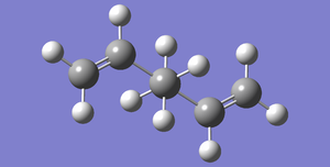Fig 1: Antiperiplanar Conformer of 1,5-Hexadiene, Total Energy: -231.69253528 a.u., Point Group: Ci
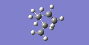Fig 2: Gauche Conformer of 1,5-Hexadiene, Total Energy: -231.69266120 a.u., Point Group: C1

From purely steric considerations, the antiperiplanar conformer was expected to be of lower energy, and therefore more stable, due to a predicted clash between the ethylene groups along the dihedral axis (SEE: Figures 1 and 2). However upon comparison of the energies, the Gauche conformer was observed to be lower in energy. Visualization of the HOMOs and LUMOs revealed a secondary π-interaction (between the π and π* orbitals respectively) exclusively within the Gauche conformer (SEE: Figures 3-8). Thus indicating a stabilizing electronic interaction that overrules any potential destabilization resulting from steric interactions.

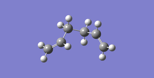Fig 3: Gauche Conformer (side on representation)
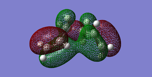Fig 4: Gauche Conformer HOMO
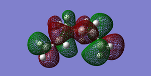Fig 5: Gauche Conformer LUMO

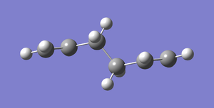Fig 6: Antiperiplanar Conformer (side on representation)
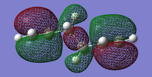Fig 7: Antiperiplanar Conformer HOMO
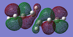Fig 8: Antiperiplanar Conformer LUMO

In addition to this π-π interaction, previous studies have also provided evidence of a CH-π interaction._[2,5] However, such an interaction was not observed in this study.

Nf710 (talk) 09:17, 11 March 2016 (UTC) Very nice use of the orbitals to explain the ordering.

Comparison of B3LYP/6-31G* to the HF/3-21G Level of Theory

The HF optimized antiperiplanar conformer was re-optimized under the B3LYP/6-31G* level of theory. Visually, this appeared to have no effect on the overall morphology of the molecule (Comparing Figures 1 and 9) . However, the energies as well as the molecular geometry (bond lengths and angles) were altered. The data regarding these findings is shown below (SEE: Figure 10). It is important to note that direct comparison of the energies across different calculation types (e.g. HF and DFT) is physically meaningless due to differences it in the theoretical constraints placed upon them.

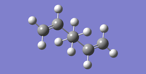Fig 9: Antiperiplanar Conformer of 1,5-Hexadiene (DFT Calculation), Total Energy: -234.61171063 Hartrees, Point Group: Ci
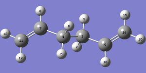Fig 10: Numbered atom diagram of Antiperiplanar 1,5-Hexadiene
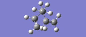Fig 11: Gauche Conformer of 1,5-Hexadiene (DFT Calculation), Total Energy: -234.61132934 Hartrees Point Group: C1
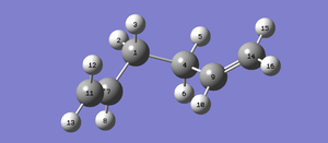Fig 12: Numbered atom diagram of Gauche 1,5-Hexadiene

Antiperiplanar Conformer Geometry

The Ci symmetry of the Antiperiplanar conformer, resulted in many of its geometric quantities being equivalent.

Bond	DFT Length / Angstroms	HF Length / Angstroms
11-7/9-14	1.33824	1.31613
7-4/1-9	1.50720	1.50891
4-1	1.55504	1.55275

Fig 13: Antiperiplanar conformer bond lengths. More variation can be seen in the C=C bonds between the two levels of theory. Indicating that the HF produces a good approximation of the σ framework, but the π system is better approximated by a higher level DFT calculation.

Angle	DFT / θ°	HF / θ°
13-11-12/15-14-16	116.291	116.310
11-7-8/14-9-10	119.213	119.680
8-7-4/10-9-1	115.563	115.507
11-7-4/14-9-1	125.220	124.806
6-4-5/3-1-2	106.708	107.715
7-4-1/9-1-4	112.648	111.349
7-4-1-9/5-4-1-3/6-4-1-2	180.000	180.000
8-7-4-5/3-1-9-10	177.177	174.269

Fig 14: Antiperiplanar conformer bond angles. Some small changes in magnitude, but the overall distribution remained the same.

Gauche Conformer Geometry

More bond lengths and angles needed to be collected, compared to the Antiperiplanar conformer, due to the lack of symmetry in the Gauche conformer (Point group: C1)

Bond	DFT or HF	Length
11-7	HF	1.31629
11-7	DFT	1.33382
7-1	HF	1.50847
7-1	DFT	1.50490
1-4	HF	1.55314
1-4	DFT	1.55013
4-9	HF	1.50929
4-9	DFT	1.50438
9-14	HF	1.31646
9-14	DFT	1.33360

Fig 15: Gauche Conformer bond lengths. The same conclusions as in Figure 13 can be drawn from here also.

Location	DFT or HF	θ°
11-7-1	HF	124.530
11-7-1	DFT	125.478
4-9-14	HF	125.024
4-9-14	DFT	124.934
7-1-4-9	HF	67.664
7-1-4-9	DFT	66.323

Fig 16: Gauche conformer bond angles.

Vibrations and Thermochemistry Data

A frequency analysis of the antiperiplanar conformer was also carried out undef the B3LYP/6-31G* regime. No imaginary frequencies were found, indicating a stable structure.

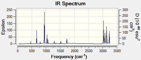Fig 17: Predicted IR Spectrum based on the analysis of the vibrations of the antiperiplanar conformer 1,5-Hexadiene

Quantity	Value
Sum of electronic and zero-point Energies	-234.469219
Sum of electronic and thermal Energies	-234.461869
Sum of electronic and thermal Enthalpies	-234.460925
Sum of electronic and thermal Free Energies	-234.500809

Fig 18: Thermochemistry data for the antiperiplanar conformer of 1,5- hexadiene. The "sum of the electronic and zero point energies" term accurately described the energy of the system at 0 K, whilst the "sum of electronic and thermal energies term" accurately describes the energy of the system at 298.15 K. These quantities were used in later calculations to determine the activation energies.

Associated Output Files

File	Description
File:OTRAP(A).LOG	HF/3-21G optimised structure of antiperiplanar 1,5-Hexadiene
File:OTRAP(B).LOG	HF/3-21G optimised structure of gauche 1,5-Hexadiene
File:OTRAP(F).LOG	B3LYP/6-31G optimised structure of antiperiplanar 1,5-Hexadiene
File:OTRAP(G).LOG	B3LYP/6-31G frequency analysis of antiperiplanar 1,5-Hexadiene
File:OTRAP(G) 0K.LOG	B3LYP/6-31G frequency analysis of antiperiplanar 1,5-Hexadiene at 0 K
File:GAUCHE 631G.LOG	B3LYP/6-31G frequency analysis of gauche 1,5-Hexadiene

Optimizing the "Chair" and "Boat" Transition Structures

The Chair and Boat transition structures were optimized using three different methods:

The Berny "Guess Structure" method
The Frozen Coordinate method
The QST2 method

Optimizing to the Chair Transition Structure (Guess Structure Method)

Two HF/3-21G optimized allyl fragments, positioned against one another in an approximate Chair-like conformation. With the end to end (where the Cope rearrangement bond breaks/forms) distances set to 2.2 Å. The structure was then optimized to the transition state (using the Berny calculation option). A frequency analysis was also carried out on the optimized structure to simulate the molecular vibrations. A single imaginary frequency was found. which corresponded directly to the molecular motion associated with the cope rearrangement. This vibration is defined as imaginary due to it's force constant value in the quantum harmonic oscillator. If the second derivative along a potential energy surface is negative at the maximum, the force constant derived will be negative. The angular frequency is obtained via: $ω = \sqrt{\frac{k}{m}}$ thus giving an imaginary output. The actual "-" is merely a notation, used by Gaussian, to define such frequencies.

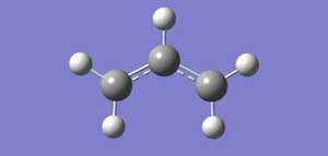Fig 19: Allyl fragment used to form half of the transition state.
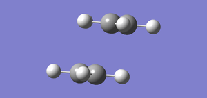Fig 20: Allyl fragments arranged to form an approximate chair structure.

Fig 21: Molecular vibration corresponding to the Cope Rearrangement (-817.62 cm^-1)

Optimizing to the Chair Transition Structure (Frozen Coordinate Method)

If the guess structure were to fail, due to the initial "guess" being far from the correct geometry, the Frozen Coordinate method may be used to correct such an error. The fragments are "frozen" at the assumed end-end distances. Each fragment is then optimized (to a minimum) around this frozen geometry to produce a structure that is closer to the desired output. The end-end coordinates are then unfrozen and optimized the the transition structure, but from a corrected starting geometry. This was attempted on the same system used in the Guess Structure.

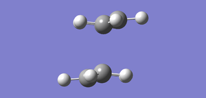Fig 22: Half-optimized Chair transition structure. The allyl fragments are optimized to a minimum whilst the end-end distance frozen at 2.2 Angstroms
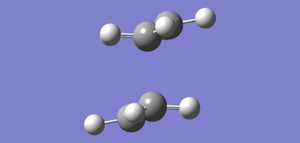Fig 23: Fully optimized Chair transition structure with the now unfrozen bonds optimized independently of the individual allyl fragments.

Upon comparison to the Guess Structure results, the Frozen Coordinate method effectively produces the same energy and and end-end distances. The Frozen Coordinate end-end distances are much similar and relate more to the expected symmetry of the transition structure. This is most likely the result of the corrected geometry of the frozen coordinate method.

Method	Energy / Hartrees	End-end distance 1 / Angstroms	End-end distance 2 / Angstroms
Guess	-231.61932209	2.01994	2.02081
Frozen Coordinate	-231.61932231	2.02071	2.02064

Fig 24: Comparison of the energies and end-end distances of the Guess Structure method and the Frozen Coordinate method.

Optimizing to the Boat Transition Structure (QST2 Method)

Although the previous calculation types may have been appropriate for the Boat structure, the QST2 method was used. This method works by specifying the reactants and products of the reaction, with each of the individual atoms labelled consistently. The transition structure is then determined by interpolating between the two structures. However, the reactant and product geometries must be carefully considered as this method does not consider the twisting of intramolecular bonds. This is demonstrated in the Boat transition structure calculations. When the simple, antiperiplanar conformer is used, the QST2 calculation did not rotate the molecule in accordance with the Cope Rearrangement. Rather, it translated one of the allyl fragments such that a Chair-like conformation is generated. In order to avoid this, the molecule was twisted manually before the calculation. This brought the molecule closer to the desired geometry. The vibrations were simulated, via a subsequent frequency analysis, giving a single imaginary frequency corresponding to the Cope Rearrangement.

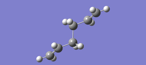Fig 25: Antiperiplanar conformer of 1,5-Hexadiene
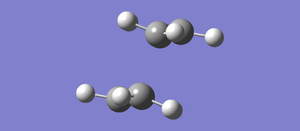Fig 26 Failed optimization to a Chair-like transition structure
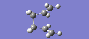Fig 27: Twisted conformer of 1,5-Hexadiene
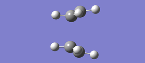Fig 28 Successful Boat transition structure

Fig 29: Molecular vibration corresponding to the Cope Rearrangement (-839.94 cm^-1)

Determining the Lowest Energy Conformer, via the Transition State, using the IRC Method

Starting from the HF optimized the Intrinsic Reaction Coordinate method (IRC) was used to find the product conformer of the Cope Rearrangement. The method works by following the slope of the potential energy surface until it finds a minimum. First an IRC calculation of 50 points was used to find the product conformer. This gave a structure that closely resembled the "Gauche 2" conformer (Energy=-231.69167, Point Group C2). Further calculations were done to ensure that this was the resulting conformer, all giving the same approximate result with some small variations. This indicates that the the Cope rearrangement does not relax back down to the "Gauche 3" conformer immediately. It must form the"Gauche 2" conformer and then rotate accordingly.

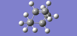Fig 30E= -231.69157910. Initial IRC calculation (50 points)

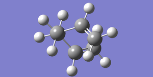Fig 31 E=-231.69166702 (IRC then subsequent HF minimisation)
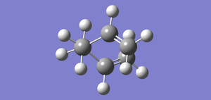Fig 32 E=-231.69157910 (IRC 110 point calculation)
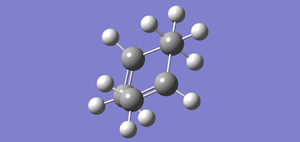Fig 33 E=-231.68295296 (IRC 50 points with force constants plotted at every step)

Re-optimizing the Chair and Boat Transition Structures via the B3LYP/6-31G* Method and Calculating the Activation Energies

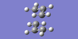Fig 34-234.55698303
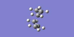Fig 35-234.54309307

Conformer	Reagent Energy (0 K) / hartrees	Reagent Energy (298.15 K) / hartrees	Transition Structure Energy (0 K) / hartrees	Transition Structure Energy (298.15 K) / hartrees	Activation Energy (0 K) / hartrees	Activation Energy (298.15 K) / hartrees
Chair HF/3-21G	-231.539539	-231.532565	-231.466701	-231.461341	0.072838	0.071224
Chair B3LYP/6-31G*	-234.469219	-234.461869	-234.414929	-234.409009	0.05429	0.05286
Boat HF/3-21G	-231.539486	-231.532646	-231.450928	-231.445299	0.088558	0.087347
Boat B3LYP/6-31G*	-234.469219	-234.461869	-234.402342	-234.396008	0.066877	0.065861

Fig 36: Activation energies calculated from Thermochemistry data. From this, it can be seen that the Chair conformer is preferred due to the lower activation energy. Comparison of the calculation methods shows that there are significant differences in the energies, leading to variable accuracy depending on which method is used. In addition, the energy trends between calculation type do not remain constant. This makes experimental comparison less facile, in terms of accuracy, between calculation types.

09:22, 11 March 2016 (UTC) You must have ran out of time here

Associated Output Files

File	Description
File:OTCABTS(A).LOG	HF/3-21G optimised allyl fragment
File:OTCABTS(B).LOG	HF/3-21G optimised chair transition structure for the Cope Rearrangement (Berny Method)
File:OTCABTS(C).LOG	HF/3-21G half-optimised chair transition structure for the Cope Rearrangement (Frozen Coordinate Method)
File:OTCABTS(D).LOG	HF/3-21G optimised chair transition structure for the Cope Rearrangement (Frozen Coordinate Method)
File:OTCABTS(E).LOG	Failed HF/3-21G optimised boat transition structure for the Cope Rearrangement (QST2 Method)
File:OTCABTS(E)-BERNY.LOG	HF/3-21G optimised boat transition structure for the Cope Rearrangement (Berny Method)
File:OTCABTS(E)TWIST.LOG	Successful HF/3-21G optimised boat transition structure for the Cope Rearrangement (QST2 Method)
File:OTCABTS(F).LOG	HF/3-21G IRC calculation for the chair transition structure (Berny) of the Cope Rearrangement
File:OTCABTS(F)I.LOG	HF/3-21G IRC output optimisation for the chair transition structure (Berny) of the Cope Rearrangement
File:OTCABTS(F)II.LOG	HF/3-21G IRC calculation for the chair transition structure (Berny) of the Cope Rearrangement (increased number of points)
File:OTCABTS(F)III.LOG	HF/3-21G IRC calculation for the chair transition structure (Berny) of the Cope Rearrangement (computing force constants at every step)
File:OTCABTS(G)-BOAT.LOG	B3LYP/631G* optimised boat transition structure
File:OTCABTS(G)-CHAIR.LOG	B3LYP/631G* optimised chair transition structure
File:OTRAP(A)-FREQ.LOG	HF frequency analysis of the 1,5 Antiperiplanar conformer of 1,5 heaxadiene
File:OTRAP(B)-FREQ.LOG	HF frequency analysis of the 1,5 Gauche conformer of 1,5 heaxadiene

The Diels-Alder Cycloaddition

The Semi-Empirical, AM1 calculation type was used for all of the folowing calculations.

Optimizing cis-Butadiene and Visualizing the HOMO and LUMO

Before forming the transition states of the Diels-Alder reaction, the two reagents: ethylene and cis-butadiene were optimized and their HOMOs and LUMOs plotted. This aided the visualization and characterization steps that followed.

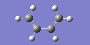Fig 37:Cis-Butadiene
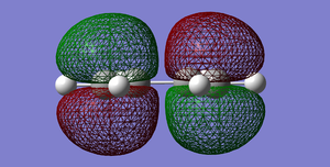Fig 38:HOMO of cis-Butadiene. Antisymmetric with respect to the plane.
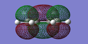Fig 39:LUMO of cis-Butadiene. Symmetric with respect to the plane

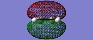Fig 40: Ethylene HOMO. Symmetric with respect to the plane.
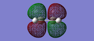Fig 41: Ethylene LUMO. Antisymmetric with respect to the plane.

Finding the Transition State Geometry of the Diels-Alder Prototype Reaction

Starting from the product and partially breaking the two reactive C-C bonds, an initial C-C guess of 2.5000 angstroms was used in a Berny optimisation of the Diels-alder reaction. The visualized MOs corresponded directly to the expected results in that the diene LUMO overlapped in phase with the dieneophile HOMO, and the dieneophile LUMO overlapped in phase with the diene HOMO. This was deduced via comparison with the reagent MOs and symmetries in the previous section. Note also that the Diels Alder reaction is a thermally allowed [4+2]-cycloaddition via Woodward-Hoffman analysis, which also explains its reactivity.

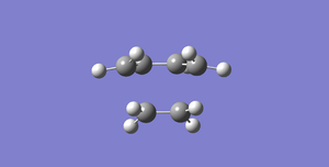Fig 42Diels-Alder Cycloaddition transition structure
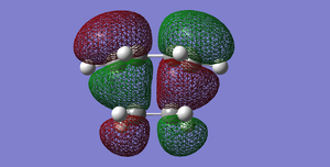Fig 43Diels-Alder Cycloaddition transition structure(HOMO). The cis-butadiene HOMO interacts with the ethylene LUMO. (Antisymmetric)
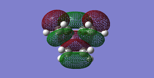Fig 44Diels-Alder Cycloaddition transition structure(LUMO). The cis-butadiene LUMO interacts with the ethylene HOMO. (Symmetric)

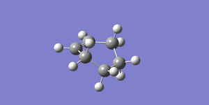Fig 45Diels-Alder Cycloaddition Product
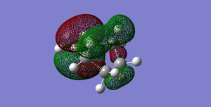Fig 46Diels-Alder Cycloaddition Product HOMO (Symmetric)
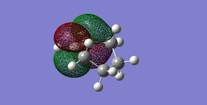Fig 47Diels-Alder Cycloaddition Product LUMO (Antisymmetric)

The vibrations of the transition structure were also simulated at the same level of theory. The imaginary, reactive vibration is shown below. The bond forming process is synchronized upon observation, as would be expected for a concerted cycloaddition reaction.

Fig 48: Molecular vibration corresponding to the Diels Alder Cycloaddition (-956.36 cm^-1, Synchronous)

In contrast, the lowest, non-imaginary vibration involves the two components oscillating in asynchronously and not in the plane of the reacting bonds, indicating why this is a non-reactive vibration. The components simply do not interact in the same plane of motion and have the wrong relative phases.

Fig 49: The lowest, positive molecular vibration corresponding to the Diels Alder Cycloaddition (147.38 cm^-1)

Bond	Length
C=C (Ethylene)	1.38297
C=C (cis-Butadiene)	1.38195 / 1.38186
C-C (cis-Butadiene)	1.39748
Partially formed C-C	2.11925 / 2.11928

Fig 50: Ethylene and cis-butadiene bond lengths. The Van der Walls radius of a Carbon atom is 1.7 Å. Therefore, the partially formed bond is shorter than 2 times this distance, indicating strong interaction within the system.

Observing the Regioselectivity of the Diels-Alder Reaction

An initial C-C guess of 2.5000 angstroms was used in a Berny optimisation of the Diels-alder reaction. This time, the ENDO/EXO transition structures were assessed using maleic annhydride and cyclohexa-1,3-diene. In the ENDO structure (and not in the EXO structure), an orbital interaction between the -(CO)-O-(CO)- π system of the dieneophile and C=C-C=C π system of the diene can be clearly visualized (SEE: Fig 52-55). This secondary orbital overlap stabilizes the transition structure. Lowering its energy, relative to the EXO transition structure, and thus explaining why the ENDO product is the kinetic product (due to the lowered relative activation energy). In addition, the energies of the ENDO and EXO products were calculated as -0.16017080 Hartrees and -0.15990915 Hartrees respectively. The lower ENDO product energy indicates that it may also be the thermodynamic product of the reaction. However, the difference in energy relatively is quite small, and it would be expected that thermal influences could nullify this influence. A steric clash with the hydrogen atoms of the $- C H_{2} - C H_{2} -$ groups above the -(CO)-O-(CO)- system may also have destabilized the EXO structure. However this interaction would have most likely been overruled by the secondary orbital overlap stabilization of the ENDO structure.

(A table with a comparison of the TS and product energies in kJ/mol or kcal/mol would be useful here Tam10 (talk) 11:42, 11 March 2016 (UTC))

The ENDO Transition State

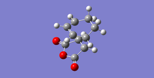Fig 51: ENDO (-0.05150480 Hartrees)
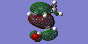Fig 52: ENDO HOMO
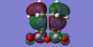Fig 53: ENDO HOMO
Fig 54: ENDO HOMO
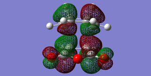Fig 55: ENDO LUMO

The EXO Transition State

Fig 56: EXO (-0.05041981 Hartrees)
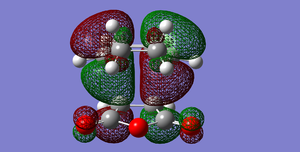Fig 57: EXO-HOMO
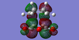Fig 58: EXO-LUMO

The reactive vibrations of this system remained largely unchanged compared to the cis-butadiene/ethylene example. A lowering of the ENDO vibration frequency further supports its position as the preferred product due to the the direct correlation between frequency and energy.

Fig 59: EXO Molecular vibration corresponding to the Cope Rearrangement (-812.22 cm^-1)

Fig 60: ENDO Molecular vibration corresponding to the Cope Rearrangement (-806.43 cm^-1)

Bond	Length (ENDO)	Length (EXO)
-C=C- (Diene)	1.39307 / 1.39306	1.39442 / 1.39439
=C-C= (Diene)	1.39725	1.39679
-C-C- (Diene)	1.52797	1.52208
-C-C= (Diene)	1.49053 / 1.49054	1.48979 / 1.48970
-C=C- (Dieneophile)	1.40850	1.41012
=C-C= (Dieneophile)	1.48923 / 1.48923	1.48818 / 1.48817
-C=O (Dieneophile)	1.22057 / 1.22057	1.22054 / 1.22054
-C-O-(Dieneophile)	1.40896 / 1.40896	1.40963 / 1.40963
r	2.16234 / 2.16242	2.17050 / 2.17024
r'	2.89221 / 2.89228	2.94495 / 2.94496

Fig 61: Bond distances for the ENDO and EXO transition structures. r and r' denote the partly formed C-C bonds and the C-C through space distances between the -(CO)-O-(CO- fragment and either the C=C unit (ENDO) or the C-C unit (EXO). Notice how the values for r and r' are smaller in the ENDO product. This further supports the concept of a secondary orbital pulling the reagents together. Thus stabilizing the transition structure, lowering the energy and shortening these distances.

Associated Output Files

File	Description
File:TDAC(I).LOG	AM1 optimised cis-butadiene
File:TDAC(II).LOG	AM1 optimised transition structure for the Diels-Alder Cycloaddition
File:TDAC(II)-PRODUCT.LOG	AM1 optimised product of the Diels Alder Cycloaddition
File:TDAC(III)-ENDO.LOG	AM1 optimised endo transition structure for the Diels-Alder Cycloaddition
File:TDAC(III)-EXO.LOG	AM1 optimised exo transition structure for the Diels-Alder Cycloaddition
File:TDAC(III)-EXO-PRODUCT.LOG	AM1 optimised exo product of the Diels Alder Cycloaddition
File:TDAC(III)-PRODUCT.LOG	AM1 optimised endo product of the Diels Alder Cycloaddition
File:ETHYLENE.LOG	AM1 optimized ethylene molecule

Conclusion

To conclude, the lowest energy conformer of 1,5-Hexadiene was found to be the "Gauche 3" conformer resulting from a π-π interaction between the terminal C=C Groups. The possible transition structures (Chair and Boat) of the Cope Rearrangement were calculated via the Berny, Frozen Coordinate and QST2 methods. It was found that the chair conformer was lower in energy and therefore the preferred transition structure. The Cope rearrangement product conformer was calculated, via IRC calculations, as the "Gauche 2" conformer. The Diels-Alder Cycloaddition was then simulated using the Berny Method. The ENDO product was found to be both the thermodynamic and kinetic product, stabilized by a secondary orbital interaction and proceeding via a synchronous molecular vibration within the transition state.

References

Charlotte Froese Fischer. General Hartree-Fock program. Computer Physics Communications 1987; 43(3): 355-365. doi:10.1016/0010-4655(87)90053-1 (accessed 22/02/2016).http://www.sciencedirect.com/science/article/pii/0010465587900531
Motohiro Nishio. CH/p hydrogen bonds in crystals. CrystEngComm 2004; 6(27): 130-158. DOI: 10.1039/b313104a (accessed 22/02/2016).http://pubs.rsc.org/en/content/articlepdf/2004/ce/b313104a.
Grimme, Stefan (2004). "Accurate description of van der Waals complexes by density functional theory including empirical corrections". Journal of Computational Chemistry 25 (12): 1463–1473. doi:10.1002/jcc.20078. (accessed 22/02/2016)
Mudar A. Abdulsattar and Khalil H. Al-Bayati. Corrections and parametrization of semiempirical large unit cell method for covalent semiconductors. Phys. Rev. B 2007; 75(245201): 1-8. DOI:http://dx.doi.org/10.1103/PhysRevB.75.245201 (accessed 22/02/2016).
BRANDON G. ROCQUE , JASON M. GONZALES & HENRY F. SCHAEFER III(2002) An analysis of the conformers of 1,5-hexadiene, Molecular Physics, 100:4, 441-446, DOI:10.1080/00268970110081412 (accessed 22/02/2016)