The Free Energy and Thermal Expansion of MgO

Introduction

This study utilized the General Utility Lattice Program (GULP) to simulate the vibrational (phonon) modes of a crystal of Magnesium Oxide (MgO). The thermal expansion of the crystal was then simulated via the Quasi Harmonic Approximation (QHA) and via molecular dynamics (MD). The free energies and lattice volumes / parameters were compared between each calculation method and the thermal expansion coefficients were calculated. Firstly some background is required to make the following calculations clear.

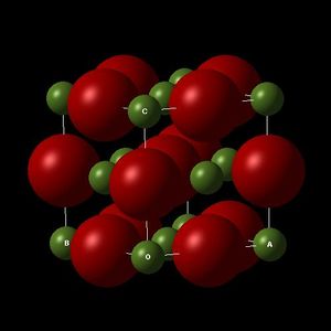MgO Conventional Lattice (FCC) Illustrating the lattice parameters a,b and c.
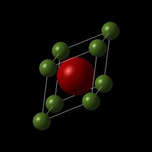MgO Primitive Lattice (Triclinic).

Reciprocal Lattice

A Fourier Transform, converts a 'real' lattice in direct (real) space into a corresponding reciprocal lattice in reciprocal space (also referred to as momentum / k space). There are several advantages to working in reciprocal space:

The Fourier coefficients associated with the conversion are related to crystallographic scattering intensities.
The reciprocal space axis system is in terms of three dimensional k-vectors which can be related to the calculation and plotting of dispersion curves and density of state graphs.
Every vibration within the crystal has an associated k-vector (in reciprocal space) that describes the direction and wavelength of the vibration.

k-vectors

In addition to its uses in reciprocal space, the k-vector can be described as the wave vector of a lattice vibrational energy level:

A 1-dimensional lattice of uniformly spaced lattice points (spacing distance 'a') would be represented by a vibrational wavefunction (Ψ) of the form:

$ψ = \sum_{n = 0}^{N} e^{- i k n a} χ_{n}$

where k is the wave vector, n is the number of lattice points in sequence, and thi is the basis function of each lattice point (e.g. a Hydrogen atom 1s orbital).

Considering that:

$k = \frac{2 π}{λ}$

when λ = 2a, k = π/a making:

$ψ = \sum_{n = 0}^{N} e^{- i π n} χ_{n} = (- 1)^{n} χ_{n}$

The relative motion of each lattice point is out-of-phase with its neighbors, producing the highest energy state.

when λ = $\infty$ , k = 0 making:

$ψ = \sum_{n = 0}^{N} χ_{n}$

The relative motion of each lattice point is in-phase with its neighbors, producing the lowest energy state.

Thus, it can be deduced that that the energy (and frequency) of the vibrational energy levels increases with k up to k = π/a (larger values of k are non unique as the wavefunction is 2π-periodic). The reqion -π/a ≤ k < π/a is known as the Brillouin zone and represents the range of unique k values in the lattice model.

Phonons

A phonon is defined as a discrete, 'collective excitation' within a periodic, elastic arrangement of atoms (such as a lattice).It is the particle representation of quantised vibrational motion inside condensed matter; in much the same way as the particle representation of light is known as a photon. It is important to note that vibrations within a crystal only occur collectively (at a specific frequency) between atoms (unlike some molecular vibrations) and is the reason why this concept is required to understand these excitations.

Dispersion Curves and the Density of States

A dispersion curve, in its simplest interpretation, can be considered as a plot of vibrational (phonon) frequencies against a predetermined range of k-values. Ideally, the range of k-values used should map the entire lattice reciprocal space (plotting across -π/a ≤ k < π/a).

The density of states (DOS) is defined as the number of vibrational levels (or states) within a given interval of energy. The DOS is normally plotted against energy or frequency, allowing facile comparison with the corresponding dispersion curve. The DOS averages over all of the k-points (not just a finite range as in the dispersion curve) within the reciprocal lattice.

Lattice Vibrations - Computing the Phonons

A Dispersion Curve across 50 k-points was computed for the MgO primitive lattice. Each continuous line of the dispersion curve represents a phonon branch. MgO is an example of a heterodiatomic lattice (Mg and O). As a result, two types of phonon branch are produced. An optical branch (Does not converge 0 cm^-1 to $Γ$ ) and an acoustic branch (Does converge at 0 cm^-1 to $Γ$ ). The labels on the k-axis are points of high symmetry in k-space and are used, as such, for reference:

Symmetry Point	k-space vectors: (x,y,z)
Gamma	0,0,0
X	0.5,0,0.5
W	0.5,0.25,0.75
L	0.5,0.5,0.5

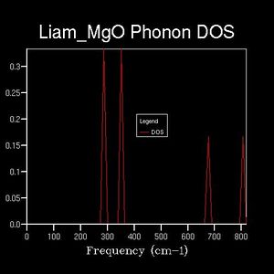
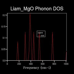
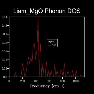
The DOS was plotted against the same frequency range as the dispersion curve, however a range of shrinking factors were tested to observe how the DOS varied. The shrinking factor determined a grid of k-points over which which the DOS average was taken. The greater the shrinking factor, the more dense the grid of k-points and thus, the greater the DOS 'resolution'. For example: the 1x1x1 reciprocal-space grid (below) plotted 1 k-point. This k-point was found by comparison with the dispersion curve. On the DOS plot, 4-peaks can be seen at different frequencies, however, the dispersion curve shows the presence of 6 branches. Therefore, the phonon mode in question must lie at a point at which two branches share the same frequency. By comparing the peak frequencies of the DOS plot with the branch frequencies of the dispersion curve, it could be seen that the k-point in question corresponded to the L-symmetry point (a value of 0.5,0.5,0.5 in reciprocal space).

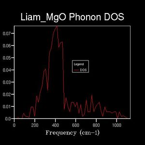
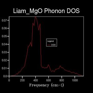
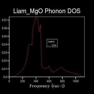
Drastic changes in the DOS could be seen upon doubling the shrinking factor (2x2x2: 4 k-points sampled). This indicated that the 1x1x1 grid was not a reasonable approximation to the true DOS. After a shrinking factor of 16x16x16, the overall distribution of the DOS remained roughly the same (aside from some smoothing of the peaks and troughs). This relates back to the concept of a more dense grid, in reciprocal space, being used at the expense of increased processing power. Thus, the minimum shrinking factor required for an adequate DOS calculation laid between 8x8x8 and 16x16x16.

1x1x1
2x2x2
4x4x4
8x8x8
16x16x16
32x32x32
64x64x64

This optimal grid size would be applicable for other compounds with the same crystal structure (CaO) but not different structures (lithium and Faujasite)

Calculating the Free Energy in the Harmonic Approximation

The above computation was repeated, with the temperature set to 300 K and the shrinking factors increased by 1 for each calculation. This produced the DOS, as before, and a corresponding Helmholtz free energy. The free energy was plotted against the shrinking factor (reciprocal space dimensions). It could be seen that the free energy increased with the shrinking factor before plateauing at a free energy of -40.926483 eV (18x18x18 shrinking factors). Thus, the minimum shrinking factor configuration for both the DOS and the free energy is 18x18x18.

However, if a lower resolution calculation would suffice, a smaller set of shrinking factors could be used:

Accurate to 1 meV: 3x3x3 (-40.926432 eV) Accurate to 0.5 meV: 4x4x4 (-40.926450 eV) Accurate to 0.1 meV: 5x5x5 (-40.926463 eV)

This optimal grid size would not be appropriate for other compounds as the bond energies would differ between them and this affect the free energy calculated.

The Thermal Expansion of MgO

Using the optimum shrinking factors (18x18x18). The variation in the free energy, the lattice parameter and the lattice volume with temperature was calculated.

The free energy decreased non-linearly with temperature. This can be rationalized by considering the definition of the Helmholtz free energy: . Where is the zero point energy. The non-linearity can be attributed to the variation in entropy with temperature under the quasi-harmonic approximation (QHA): $S (V) = - \frac{1}{N} \sum_{k, i} k_{B} \ln [1 - \exp (- \frac{h ν_{k, i} (V)}{k_{B} T})] + \frac{1}{N} \sum_{k, i} k_{B} \frac{h ν_{k, i} (V)}{k_{B} T} {[\exp (- \frac{h ν_{k, i} (V)}{k_{B} T}) - 1]}^{- 1}$

Note that the QHA approximates the difference in the variation in lattice parameter/volume as a parabola. Thus (much like its relation to the Lennard-Jones potential) the QHA is only accurate at displacements close to equilibrium. Therefore at very high temperatures (e.g. the MgO melting point) the QHA doesn't accurately represent the motion of the lattice as it does not take bond dissociation into account and instead, assumes the lattice bonds increase indefinitely with energy (temperature). The lattice parameter/volume increased non-uniformly with the temperature. This was due to the nature of thermal expansion under the QHA: $α_{V} = \frac{1}{V} {(\frac{\partial V}{\partial T})}_{P}$

The physical significance of this equation can be derived intuitively by imagining a cube of volume V. Upon heating, the cube volume increases by dV. The magnitude of the expansion is characterized by the thermal expansion coefficient () which varies between materials and temperatures.

In order to find the expansion coefficient the curve was approximated using a polynomial expansion:

$V = 3 x 1 0^{- 07} T^{2} + 0.0002 T + 18.823$

${(\frac{\partial V}{\partial T})}_{P} = 6 x 1 0^{- 07} T + 0.0002$

$α_{V} = \frac{1}{V} (6 x 1 0^{- 07} T + 0.0002)$

Molecular Dynamics

The thermal expansion was simulated once again, but instead of the QHA, molecular dynamics (MD) calculations were used. The main distinction between the two methods is that MD uses classical mechanics to run calculations, whereas the QHA uses quantum mehanics. In this case, the conventional MgO supercell lattice was used which contained 32 MgO units, hence the data from the QHA needed to be multiplied by 32 in order to make a valid comparison between the two calculation types. A supercell is used for MD calculations as the traditional primitive cell (used for QHA) would result in totally in phase motion, due to the presence of a single MgO unit, which would not simulate the system effectively.

The MD free energy and lattice volume calculations both produced linear distributions against temperature and had no vales at 0 K; this was again, due to the classical interpretation. Hence there was no zero-point energy value associated with 0K, unlike in the QHA. This makes the QHA more valid at low temperatures and MD at high temperatures. However, neither are good approximations for phase transitions (i.e. melting points) as they do not take these into account. Lattice volumes under MD increase linearly with temperature, whilst the QHA remains parabolic throughout.