Rep:Mod:LISIMSns2214

Simulation of Simple Liquids

Introduction

Molecular dynamics simulations simplifies measuring properties of a material and constructing further calculations. A computer is able to calculate these properties by taking into account the individual atomic environments within the material. This can be vastly complicated with even the most simple liquid systems, but HPC (High Performance Computing) can analyse complex structures and dynamics such as protein folding.

Visual Molecular Dynamics (VMD) was used to collate and visualise the trajectory files created by Large-scale Atomic/Molecular Massively Parallel Simulator (LAMMPS) software. In order to analyse and predict properties of the system, a number of constraints and approximations had to be made. These included approximations based upon the classical harmonic oscillator, placing the medium within a box and working under ensembles. The system was then equilibrated through modifying parameters such as time-step. Phase diagrams were studied to determine pressures and densities that fell under the solid, liquid and gaseous phases, pressures were altered and heat capacities calculated. Finally, the structures of different phases of the material were confirmed through radial distribution functions (RDF) and diffusion coefficients were calculated to study how atoms within the boundaries moved about.

Introduction to molecular dynamics simulation

In order to simulate a system even as basic as a simple liquid, there are several constraints. One main assumption is that the atoms within a liquid behave classically and the system. In a liquid, the atoms can translate and experience forces between each other, i.e. a N-atom system with N force equations. Another approximation made is that there are solely pair potentials, meaning that the potential energy is assumed to only exist between pairs of atoms within the liquid- this is the basis of the Lennard-Jones Potential used to calculate Van Der Wahl's interactions. Time is no longer considered a continuous entity and split into small defined time-steps, forming the Verlet algorithm. This predicts the position of atoms based on the previous time-step positions and does not depend on the particles' velocities in previous time-steps.

Velocity can be integrated into the Verlet algorithm in order to determine energies of the system (Velocity-Verlet algorithm). It is assumed that the change in acceleration between the two time-steps is small enough that the average acceleration can be taken from the mean of the initial and final time-steps. There is a certain amount of error associated with approximations and from numerical integrations, which can be minimised with the correct time-step values and other parameters.

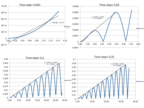
Five simulations were run at different time-steps ranging from 0.001-0.015 s. The position of the particle was based on the harmonic oscillator approximation $x\left(t\right)=A\cos (\omega t+\varphi )$ where $A=1$, $\omega =1$ and $\varphi =0$. The total energy was calculated as the sum of the kinetic $K=\frac{1}{2}m{v}^2$ and potential $U=\frac{1}{2}k{x}^2$ energies, where $m=k=1$ . In addition, error analysis was conducted by plotting the absolute difference between the values obtained from the classical harmonic approximation and Velocity-Veret solution: ${\mathbf{v}}_i(t+\delta t)={\mathbf{v}}_i(t+\frac{1}{2}\delta t)+\frac{1}{2}{\mathbf{a}}_i(t+\delta t)\delta t$ where v(0)= 0 and x(0)= 1.

Figure 1 Graphs showing Displacement vs Time (Top), Energy vs. Time (Middle), Error vs. Time (Bottom)

Error maxima found at: (2.90,0.0007585), (4.90,0.0020077), (8.000.0033008), (11.10,0.0046039) and (14.20,0.0059105) at time-step 0.001.

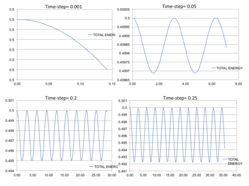
It can be seen that the displacement and (Figure 1 (Top)) of the particle oscillates from -1 to +1. The energy of the particle, much like the position, oscillates with time between 0.5000 and 0.4988 as the regular time-steps create a cycle. The displacements suggest that the classical harmonic oscillator is a reasonable approximation to make as the values behave accordingly. However, the total energy of the system fluctuates at different time-steps which is a deviation from the classical harmonic approximation, as there should be constant frequency throughout. The total average therefore needs to be constant, even if there are fluctuations, so the energy total is conserved and the simulation is valid. The increase in time-step increases the oscillation range as there are longer time periods between measurements. Because of these deviations early on is our studies, it is important to analyse the error present at this time-step and modify the parameters to minimise this. At a time-step of 0.01s (Figure 1 (Bottom)), it can be seen that the error increases with increasing time-step, so the deviation from classical increases and the approximation becomes less accurate. The gradient of the linear error trend-line increases with increasing time-step, confirming that errors and deviation are more prevalent here.

Altering the time-step affected the energy and error plots significantly. Too high a time-step creates deviations that cannot be considered fluctuations anymore. The time-step had to be kept under 0.2 to ensure an error deviation of less than 1% (±0.005) and therefore further calculations based on this time-step or below are valid. The error plots for displacement calculations are also lower with decreasing time-step value, which is favourable.

Figure 2. Graphs showing the reduced energy as a function of time with varying time-steps

Figure 3. Graph showing the erroras a function of time with varying time-steps

$\varphi \left(r\right)=4ϵ(\frac{{\sigma }^{12}}{r^{12}}-\frac{{\sigma }^6}{r^6})$

${\mathbf{r}}_{\mathbf{0}}$ when potential energy is zero:

$\frac{{\sigma }^{12}}{{r_0}^{12}}-\frac{{\sigma }^6}{{r_0}^6}=0$

$\frac{{\sigma }^{12}}{{r_0}^{12}}=\frac{{\sigma }^6}{{r_0}^6}$

$\frac{{\sigma }^{12}{r_0}^6}{{r_0}^{12}{\sigma }^6}=1$

$\frac{{\sigma }^6}{{r_0}^6}=1$

${\sigma }^6={r_0}^6$

$\sigma =r_0$

Force expereinced at ${\mathbf{r}}_{\mathbf{0}}$: ${\mathbf{F}}_0=-\frac{\mathrm{d}\varphi \left({\mathbf{r}}^0\right)}{\mathrm{d}{\mathbf{r}}_i}$

${\mathbf{F}}_0=-(-4$x$12ϵ\left(\frac{{\sigma }^{12}}{{r_0}^{13}}\right)+4$x$6ϵ\left(\frac{{\sigma }^6}{{r_0}^7}\right))$

${\mathbf{F}}_0=-(-48ϵ\left(\frac{{\sigma }^{12}}{{r_0}^{13}}\right)+24ϵ\left(\frac{{\sigma }^6}{{r_0}^7}\right))$

${\mathbf{F}}_0=-(-48ϵ\left(\frac{1}{r_0}\right)+24ϵ\left(\frac{1}{r_0}\right))$

${\mathbf{F}}_0=-(-48ϵ\left(\frac{1}{\sigma }\right)+24ϵ\left(\frac{1}{\sigma }\right))$

${\mathbf{F}}_0=\frac{24ϵ}{\sigma }$

Equilibrium separation ${\mathbf{r}}_{\mathbf{e}\mathbf{q}}$ is when ${\mathbf{F}}_0=0$ :

$-48ϵ\left(\frac{{\sigma }^{12}}{{r_{eq}}^{13}}\right)+24ϵ\left(\frac{{\sigma }^6}{{r_{eq}}^7}\right)=0$

$24ϵ\left(\frac{{\sigma }^6}{{r_{eq}}^7}\right)=48ϵ\left(\frac{{\sigma }^{12}}{{r_{eq}}^{13}}\right)$

$\left(\frac{{\sigma }^6}{{r_{eq}}^7}\right)=2\left(\frac{{\sigma }^{12}}{{r_{eq}}^{13}}\right)$

$1=\frac{2{\sigma }^6}{{r_{eq}}^6}$

$r_{eq}=2^{\left(\frac{1}{6}\right)}\sigma$

Well Depth $\varphi \left(r_{eq}\right)$:

$\varphi \left(r_{eq}\right)=4ϵ(\frac{{\sigma }^{12}}{{r_{eq}}^{12}}-\frac{{\sigma }^6}{{r_{eq}}^6})$ =$4ϵ(\frac{{\sigma }^{12}}{4{\sigma }^{12}}-\frac{{\sigma }^6}{2{\sigma }^6})$ =$4ϵ(\frac{1}{4}-\frac{1}{2})$ =$-ϵ$

Evaluation of $\underset{2\sigma }{\overset{\mathrm{\infty }}{\int }}\varphi \left(r\right)\mathrm{d}r$when $\sigma =ϵ=1.0$ :

$\underset{2\sigma }{\overset{\mathrm{\infty }}{\int }}4ϵ(\frac{{\sigma }^{12}}{r^{12}}-\frac{{\sigma }^6}{r^6})\mathrm{d}r=4ϵ(\frac{{\sigma }^{12}}{-11r^{11}}-\frac{{\sigma }^6}{-5r^5})$

=${4(\frac{-1}{11r^{11}}+\frac{1}{5r^5})|}_{2\sigma }^{\mathrm{\infty }}$

=$0-4(\frac{-1}{11*2^{11}}+\frac{1}{5*2^5})$= -0.0252

Evaluation of $\underset{2.5\sigma }{\overset{\mathrm{\infty }}{\int }}\varphi \left(r\right)\mathrm{d}r$when $\sigma =ϵ=1.0$ :

$\underset{2.5\sigma }{\overset{\mathrm{\infty }}{\int }}4ϵ(\frac{{\sigma }^{12}}{r^{12}}-\frac{{\sigma }^6}{r^6})\mathrm{d}r=4ϵ(\frac{{\sigma }^{12}}{-11r^{11}}-\frac{{\sigma }^6}{-5r^5})$

=${4(\frac{-1}{11r^{11}}+\frac{1}{5r^5})|}_{2.5\sigma }^{\mathrm{\infty }}$

=$0-4(\frac{-1}{11*2.5^{11}}+\frac{1}{5*2.5^5})$= -0.00820

Evaluation of $\underset{3\sigma }{\overset{\mathrm{\infty }}{\int }}\varphi \left(r\right)\mathrm{d}r$ when $\sigma =ϵ=1.0$ :

$\underset{3.0\sigma }{\overset{\mathrm{\infty }}{\int }}4ϵ(\frac{{\sigma }^{12}}{r^{12}}-\frac{{\sigma }^6}{r^6})\mathrm{d}r=4ϵ(\frac{{\sigma }^{12}}{-11r^{11}}-\frac{{\sigma }^6}{-5r^5})$

=${4(\frac{-1}{11r^{11}}+\frac{1}{5r^5})|}_{3\sigma }^{\mathrm{\infty }}$

=$0-4(\frac{-1}{11*3.0^{11}}+\frac{1}{5*3.0^5})$= -0.00329

Estimate the number of water molecules in 1ml of water under standard conditions. Estimate the volume of 10000 water molecules under standard conditions :

1ml~ 1g/cm^-3; number of molecules= moles x Avogadro's number = mass x N_A/molar mass

=$\left(\frac{1}{2(1.01)+16}\right)$ x 6.02 x 10²³= 3.34 x 10²²

Volume of 10000 water molecules under standard conditions:

moles= number of molecules/ Avogadro's number= 10000/N_A= 1.66 x 10^-20 mol

mass = moles x molar mass= (1.66 x 10^-20) x (18.02) = 2.99 x 10^-19 g

$Volume=\frac{m}{\rho }=\frac{2.99\mathrm{x}10^{-}19}{1}$ = 2.99 x 10^-19 ml

Working with reduced units allows for simplified calculations :

The medium is contained within a box-like system, where if the displacement extends beyond the dimensions of the box, a replicate atom enters via the opposite face. For instance, an atom at position $(0.5,0.5,0.5)$ can be placed in a cubic simulation box which runs from $(0,0,0)$ to $(1,1,1)$. If it moves along the vector $(0.7,0.6,0.2)$ in a single time-step, it will end up at: $(0.2,0.1,0.7)$ .

Leonard-Jones parameters for the element Argon are: $\sigma =0.34nm$ and $(\frac{ϵ}{K_B})=120K$

$r=(r^{*})/sigma=3.2(0.34)$= 1.09 nm

$T=\frac{1.5(120(K_B))}{(K_B)}$ = 1.5 x 120= 180 K

$$\begin{gathered} -ϵ \\ / \\ {k}_B=-120 \end{gathered}$$

$$\begin{gathered} -ϵ \\ =-120k_B \end{gathered}$$ = -0.998 kJmol^-1

Equilibration

Having placed the simulation in a box with periodic boundaries, it is essential that the system reaches equilibrium and the parameters can be modified accordingly to ensure this. In a liquid, there is no long range order. An initial idea would be to generate random co-ordinates for the atoms in the box but this brings its own set of problems. If two atoms happen to be generated so they're close in space together, there will be a lot of repulsive interactions , increasing the potential energy dramatically. In an harmonic oscillator , it is assumed that the total energy remains constant so this spike in potential energy will effectively break the approximation and create more error in the simulation values.

In order to overcome this issue, the atoms are given starting co-ordinates of cubic structures such as Face-Centred Cubic (FCC) or Simple Cubic (SC). The size of the box can be restricted in the input file, where in the line 'lattice,' the crystal structure type and the number density can be specified. For instance this line in the input file

lattice sc 0.8

would generate a box of length 1.07722. In a simple cubic structure, there in only one lattice point per unit cell:

$$\begin{gathered} \frac{\mathrm{N}\mathrm{u}\mathrm{m}\mathrm{b}\mathrm{e}\mathrm{r} \\ \mathrm{o}\mathrm{f} \\ \mathrm{l}\mathrm{a}\mathrm{t}\mathrm{t}\mathrm{i}\mathrm{c}\mathrm{e} \\ \mathrm{p}\mathrm{o}\mathrm{i}\mathrm{n}\mathrm{t}\mathrm{s}}{\mathrm{V}\mathrm{o}\mathrm{l}\mathrm{u}\mathrm{m}\mathrm{e}}=0.8 \end{gathered}$$

$$\begin{gathered} \frac{\mathrm{N}\mathrm{u}\mathrm{m}\mathrm{b}\mathrm{e}\mathrm{r} \\ \mathrm{o}\mathrm{f} \\ \mathrm{l}\mathrm{a}\mathrm{t}\mathrm{t}\mathrm{i}\mathrm{c}\mathrm{e} \\ \mathrm{p}\mathrm{o}\mathrm{i}\mathrm{n}\mathrm{t}\mathrm{s}}{0.8}=\mathrm{V}\mathrm{o}\mathrm{l}\mathrm{u}\mathrm{m}\mathrm{e} \end{gathered}$$

$\frac{1}{0.8}=\mathrm{V}\mathrm{o}\mathrm{l}\mathrm{u}\mathrm{m}\mathrm{e}$

$(\frac{1}{0.8}{)}^{\frac{1}{3}}=\mathrm{S}\mathrm{i}\mathrm{d}\mathrm{e}\mathrm{l}\mathrm{e}\mathrm{n}\mathrm{g}\mathrm{t}\mathrm{h}$

$\mathrm{S}\mathrm{i}\mathrm{d}\mathrm{e}\mathrm{l}\mathrm{e}\mathrm{n}\mathrm{g}\mathrm{t}\mathrm{h}\mathrm{=}\mathrm{1}\mathrm{.}\mathrm{0}\mathrm{7}\mathrm{7}\mathrm{2}\mathrm{2}$

If instead a FCC structure was used to generate initial position co-ordinates, with a number density of of 1.2, there would be 4 lattice points in the unit cell:

$$\begin{gathered} \mathrm{N}\mathrm{u}\mathrm{m}\mathrm{b}\mathrm{e}\mathrm{r} \\ \mathrm{o}\mathrm{f} \\ \mathrm{l}\mathrm{a}\mathrm{t}\mathrm{t}\mathrm{i}\mathrm{c}\mathrm{e} \\ \mathrm{p}\mathrm{o}\mathrm{i}\mathrm{n}\mathrm{t}\mathrm{s}=\frac{1\mathrm{x}8}{8}+\frac{1\mathrm{x}6}{2}=4 \end{gathered}$$

$$\begin{gathered} \frac{\mathrm{N}\mathrm{u}\mathrm{m}\mathrm{b}\mathrm{e}\mathrm{r} \\ \mathrm{o}\mathrm{f} \\ \mathrm{l}\mathrm{a}\mathrm{t}\mathrm{t}\mathrm{i}\mathrm{c}\mathrm{e} \\ \mathrm{p}\mathrm{o}\mathrm{i}\mathrm{n}\mathrm{t}\mathrm{s}}{\mathrm{V}\mathrm{o}\mathrm{l}\mathrm{u}\mathrm{m}\mathrm{e}}=1.2 \end{gathered}$$

$$\begin{gathered} \frac{\mathrm{N}\mathrm{u}\mathrm{m}\mathrm{b}\mathrm{e}\mathrm{r} \\ \mathrm{o}\mathrm{f} \\ \mathrm{l}\mathrm{a}\mathrm{t}\mathrm{t}\mathrm{i}\mathrm{c}\mathrm{e} \\ \mathrm{p}\mathrm{o}\mathrm{i}\mathrm{n}\mathrm{t}\mathrm{s}}{1.2}=\mathrm{V}\mathrm{o}\mathrm{l}\mathrm{u}\mathrm{m}\mathrm{e} \end{gathered}$$

$\frac{4}{1.2}=\mathrm{V}\mathrm{o}\mathrm{l}\mathrm{u}\mathrm{m}\mathrm{e}$

$(\frac{4}{1.2}{)}^{\frac{1}{3}}=\mathrm{S}\mathrm{i}\mathrm{d}\mathrm{e}\mathrm{l}\mathrm{e}\mathrm{n}\mathrm{g}\mathrm{t}\mathrm{h}$

$\mathrm{S}\mathrm{i}\mathrm{d}\mathrm{e}\mathrm{l}\mathrm{e}\mathrm{n}\mathrm{g}\mathrm{t}\mathrm{h}\mathrm{=}\mathrm{1}\mathrm{.}\mathrm{4}\mathrm{9}\mathrm{3}\mathrm{8}\mathrm{0}$

The next few lines in the input script define the volume of space, i.e the number of unit cells. The line

region box block 0 10 0 10 0 10
create_box 1 box

generates 10x10x10 unit cells and so if the simulation were based upon a FCC structure, the number of lattice spacings would be (10x10x10)x4= 4000.

The purpose of the following commands in the input script

mass 1 1.0

1 type of atom each with a mass of 1.0.

pair_style lj/cut 3.0

Lennard-Jones potential pair energy interactions where the cut ff point is 3.0, beyond this distance there are no interactions.

pair_coeff * * 1.0 1.0

Dictates the field coefficients for all pairs of atom types.

As ${\mathbf{x}}_i\left(0\right)$ and ${\mathbf{v}}_i\left(0\right)$ are specified, the Velocity-Verlet algorithm can be used for integration.

Before running the simulation, a time-step needs to be dictated in the input file, which coincides and agrees with the box constraints placed upon the liquid. It is important to set the time-step under a variable so that regardless of the time-step value, the simulations run for the same lengths of times and can be compared. If only the time-steps and runs were stated, they simulations would run for shorter lengths of time with shorter time-steps.

Figure 4. Graph showing the reduced energy as a function of time using a timestep of 0.001s

Figure 5. Graph showing the reduced temperature as a function of time using a timestep of 0.001s

Figure 6. Graph showing the pressure as a function of time using a timestep of 0.001s

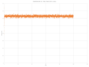
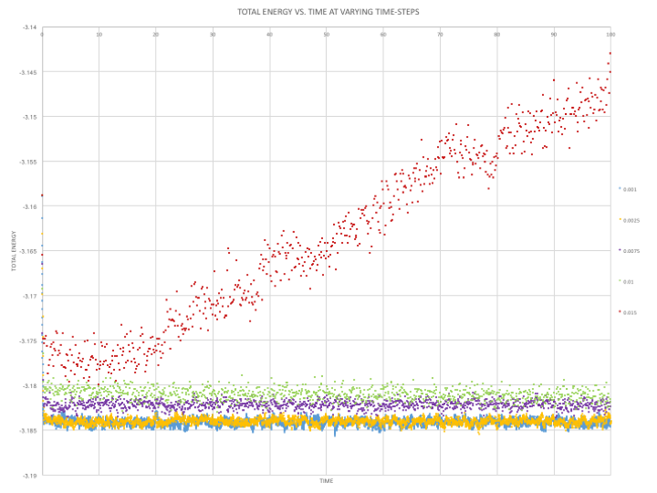
The simulation is at equilibrium at a time-step of 0.001 and the graphs of total energy, temperature and pressure show that the medium reaches the equilibrium zone within a few time-steps. The problem with a shorter time-step is that even though accurate results are obtained, they are only recorded for a shorter amount of time. This simulation requires observation over an extended period of time in order to allow the initial FCC or SC co-ordinates to arrange themselves into likely configurations.

As can be seen in Figure 4, the simulation at a time-step of 0.01 is the largest time-step to give acceptable results, where the total energy begins to fluctuate around a value of -3.81. However at this time-step, there is a large amount of fluctuation, as can be seen by the large scatter of data values.

A time-step of 0.015 gives a particularly bad result, as the energy does not equilibrate in the time period and shows no signs of doing so. The average value will therefore not be constant and an inaccurate representation of the system's energy. It is vital that the total energy of the system reaches a fluctuation zone as the simulation has been placed in a box-like space and under the ensemble (N,V,E). At this time-step the constraint is not in place.

A compromise between accuracy and time length can be made with the time-step of 0.0025. There is minimal fluctuation and scatter of values, but also allows enough time for the particles in the system to be randomly dispersed, much like a liquid would be.

Figure 7 Graph Showing Total Energy VS. Time at Varying Time-Steps

Running Simulations Under Specific Conditions

In this section the ensemble is transformed from microcanonical (N,V,E) to isobaric-isothermal (NpT) in order to investigate simulations under these conditions. 10 simulations were run at temperatures ranging from 1.75-2.75 and at pressures of 0;2 and 0.8. The temperature tends to fluctuate in the system as the atoms interact in the box, however this can be made constant by altering the volume at each time-step. The constant $\gamma$ can be applied to the kinetic energy of the system, which will effectively alter the temperature so it remains constant.

$E_K=\frac{3}{2}N{k}_{B}T$

$\frac{1}{2}\sum _i{m}_i{v}_i^2=\frac{3}{2}N{k}_{B}T$

$\frac{1}{2}\sum _i{m}_i{\left(\gamma v_i\right)}^2=\frac{3}{2}N{k}_B\mathfrak{𝔗}$

$\frac{3}{2}N{k}_B=\frac{1}{2\mathfrak{𝔗}}\sum _i{m}_i{\left(\gamma v_i\right)}^2=\frac{1}{2T}\sum _i{m}_i{v}_i^2$

$\frac{1}{2\mathfrak{𝔗}}\sum _i{m}_i(\gamma {)}^2{v}_i^2=\frac{1}{2T}\sum _i{m}_i{v}_i^2$

${\gamma }^2=\frac{\frac{1}{2T}\sum _i{m}_i{v}_i^2}{\frac{1}{2\mathfrak{𝔗}}\sum _i{m}_i{v}_i^2}$

${\gamma }^2=\frac{\mathfrak{𝔗}}{T}$

$\gamma =$±$\sqrt{\frac{\mathfrak{𝔗}}{T}}$

Towards the end of the input file, the lines dictate which properties of the system are recorded and averages them.

### MEASURE SYSTEM STATE ###
thermo_style custom step etotal temp press density
variable dens equal density
variable dens2 equal density*density
variable temp equal temp
variable temp2 equal temp*temp
variable press equal press
variable press2 equal press*press
fix aves all ave/time 100 1000 100000 v_dens v_temp v_press v_dens2 v_temp2 v_press2
run 100000

The '100' '1000' and '100000' in the penultimate line are N_every N_repeat and N_frequency respectively:

N_every is the frequency of values used from the input file, i.e. every hundred time-steps

N_repeat is the number of values from the input file used for averaging, here it's 1000 atoms

N_frequency dictates after how many time-steps the average is calculated, 100000 time-steps

Figure 8 Graphs displaying density vs. temperature at different pressures

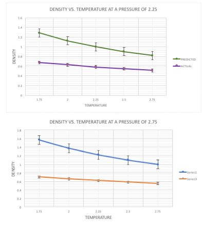
The densities generated by the simulation can be compared with those calculated based on the ideal gas law. At both pressures it can be seen that the predicted densities are almost double that of the simulated densities. The main assumption in the ideal gas law is that there are no interatomic interactions, which are accounted for in the Lennard-Jones simulation. The lack of repulsive forces means that the atoms can be close together in the prediction with no expense of potential energy, thus the density is higher. There is a larger difference between the predicted and actual values at the higher pressure of 2.75. The predicted values increase linearly as the pressure is increased (pV=nRT), however with the actual values, this is not the case. The interatomic attractions and repulsions mean that the density doesn't increase as much as the predicted values do, causing the gap expansion in values.

Calculating Heat Capacities Using Statistical Physics

The simulations were run under a density-temperature phase in order to calculate the heat capacity. A temperature range of 2-2.8 and pressures of 0.2 and 0.8 were used. The magnitude of fluctuations in the system can inform us of the heat capacity of the material, which can be plotted as a variance of the energy against temperature.

The following input script was used, varying the temperature and density

### SPECIFY THE REQUIRED THERMODYNAMIC STATE ###
variable T equal 2.0
variable D equal 0.2
variable timestep equal 0.0025

### DEFINE SIMULATION BOX GEOMETRY ###
lattice sc ${D} 
region box block 0 15 0 15 0 15
create_box 1 box
create_atoms 1 box

### DEFINE PHYSICAL PROPERTIES OF ATOMS ###
mass 1 1.0
pair_style lj/cut/opt 3.0
pair_coeff 1 1 1.0 1.0
neighbor 2.0 bin

### ASSIGN ATOMIC VELOCITIES ###
velocity all create ${T} 12345 dist gaussian rot yes mom yes

### SPECIFY ENSEMBLE ###
timestep ${timestep}
fix nve all nve

### THERMODYNAMIC OUTPUT CONTROL ###
thermo_style custom time etotal temp press
thermo 10

### RECORD TRAJECTORY ###
dump traj all custom 1000 output-1 id x y z

### SPECIFY TIMESTEP ###

### RUN SIMULATION TO MELT CRYSTAL ###
run 10000
unfix nve
reset_timestep 0

### BRING SYSTEM TO REQUIRED STATE ###
variable tdamp equal ${timestep}*100
fix nvt all nvt temp ${T} ${T} ${tdamp} 
run 10000
reset_timestep 0
unfix nvt
fix nve all nve

### MEASURE SYSTEM STATE ###
thermo_style custom step etotal temp atoms vol 
variable energy equal etotal
variable energy2 equal etotal*etotal
variable temp equal temp
variable temp2 equal temp*temp
variable n equal atoms
variable n2 equal atoms*atoms
variable vol equal vol
fix aves all ave/time 100 1000 100000 v_energy v_temp v_energy2 v_temp2
run 100000

variable aveenergy equal f_aves[1]
variable avetemp equal f_aves[2]
variable aveenergy2 equal f_aves[3]
variable ave2energy equal f_aves[1]*f_aves[1]
variable heatcap equal (${n2}*(${aveenergy2}-${ave2energy})/(${avetemp}*${avetemp}))
variable heatcapperunitvolume equal (${n2}*(${aveenergy2}-${ave2energy})/(${avetemp}*${avetemp}))/${vol}

print "Averages"
print "--------"
print "Temperature: ${avetemp}"
print "Heat Capacity: ${heatcap}"
print "Heat Capacity Per Unit Volume: ${heatcapperunitvolume}" 

Figure 9 Graphs displaying heat capacity vs. temperature at different densities

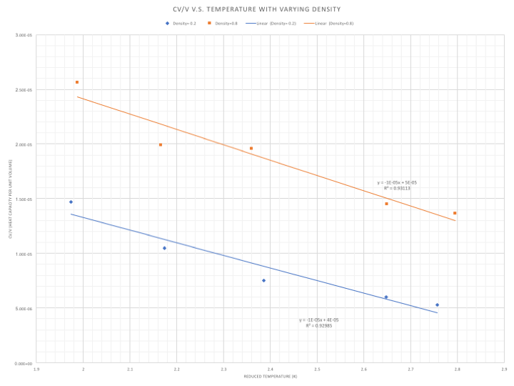
The general trend displayed in Figure 8 is that as the temperature increases, the heat capacity decreases- a system at a higher temperature requires less energy to be heated incrementally than a system at a lower temperature. This is because the density of states is larger at a higher temperature system and less energy is needed to move up the vibrational states, which are closer together. In addition the particles are further apart at a higher temperature and so fewer interatomic interactions take place, increasing the energy put towards heating the system instead of overcoming repulsive forces, thus lowering the heat capacity.A more dense system has a higher heat capacity as a result of the larger number of particles per unit volume. In a more dense system, more energy has to be applied to heat the particles to the same extent as a less dense system, increasing the heat capacity directly. With an increasing number of particles, there is also more degrees of vibrational freedom and more lost pathways.

Radial Distribution Function

Plotting the radial distribution functions of a simulated medium can give insight into the positioning of atoms relative to each other. It is also a way of confirming that the force field coefficients are in place in the LJ type system.

Figure 10graph showing how radial distribution varies with distance

Figure 11 Integration of radial distribution along increasing distance

In order to analyses the radial distributions of the sample in three phases, the density and temperature parameters had to be altered so they fell in the correct phase boundaries. These were the following values used according to the phase diagram for the Lennard-Jones potential system  :

Solid Temp= 0.75 Density= 1.2

Liquid Temp= 1.2 Density= 0.8

Gas Temp= 1.2 Density= 0.03

The radial distribution for the solid phase shows long-range ordering, as there are nearest neighbours from the first co-ordinate. The first peak corresponds to the co-ordinate of an atom from which the neighbours are displayed relative to it:

(1.025 5.29) nn= 12-0= 12

(1.475 1.13) nnn= 18-12= 6

(1.825 3.28) snnn= 42-18= 24

The co-ordinates displayed for the solid phase are roughly periodic with distance (~distance= 0.425) confirming the regular lattice structure with the applied temperature and density parameters. There are defects present in the solid structure seen at (2.125, 1.173378937) and these are sue to statistical errors as a results of the rigid system.

In a liquid however, these defects are smoothed out in the dynamic averaging. There is no long range ordering as the atoms translate over each other. The RDF quickly fluctuates around 1 after r= 2.225 as beyond this distance, there are no neighbours. The gas displays no nearest neighbours as the atoms are very far apart and with n long range ordering. Only the initial co-ordinate is recorded in the distance under which the simulation is recorded.

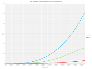
Looking at the RDF integrals, the solid has the greatest area under the curve due to its regular structure where the particles are close to one another. Looking from a point reference atoms, there are lattices extending from every dimension and so the integral increases exponentially. With liquids, there is some long range ordering so the integral also increases but at a slower rate. The gaseous phase has the lowest density and no ordering so as the particles are far apart, it's difficult to come across one along a distance and the area under the curve is small.

Dynamic Properties and Diffusion Coefficient

The diffusion coefficient is a useful form in which to study the extent to which atoms move around in a simulation and can be calculated via two methods. One way is through the means square displacement which measures the difference between the position of a particle and a reference position in the box. Another method is to use the velocity autocorrelation function where the velocity of an atom does not depend on its velocity several time-steps ago, i.e. the movement is dynamic and irregular. The phase conditions from the previous section were used to simulate the solid, liquid and gaseous phases in the smaller system.

Figure 12 Graph showing MSD vs. average time-step for solid phase (time-step= 0.002)

Figure 13 Graph showing MSD vs. average time-step for liquid phase (time-step= 0.002)

Figure 14Graph showing MSD vs. average time-step for gas phase (time-step= 0.002)

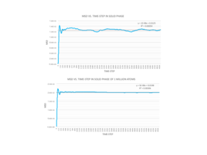
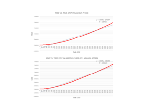
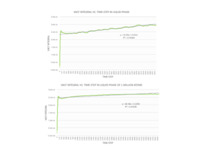
Figures 12,13 and 14 display the MSD vs. average time-step for the three phases. In the solid phases, the MSD quickly shoots up and then proceeds to fluctuate around a particular value; In the small system of 8000 atoms and large system of 1 million atoms, its fluctuates around a value of 0.0014 and 0.02 respectively. The difference in the displacement becoming a constant value within a few time-steps confirms the rigidity of the structure created, where the atoms have remained in a lattice structure due to to the temperature and pressure conditions.

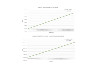
Once the temperature and pressure values are altered to allow for liquid and vapour phases, it can be seen that the MSD increases roughly linearly with time. This implies that there are particles at several different positions from the reference position and that they are dispersed randomly with no structure. The gradient for the vapour phase is almost 40 times larger than the gradient for the liquid phase as there are infinitely more degrees of freedom as you move from the liquid to gaseous phase. A liquid may not have long range ordering, but the particles are much closer and translate over each other, whereas in a gas the particles are further apart and no ordering at all. This explains the slight curve at the beginning of the gaseous graphs, where no particles are found within the first few time-steps as they are so far apart.

The diffusion coefficients below in table were calculated using the formula $D=\frac{1}{6}\frac{\partial ⟨r^2\left(t\right)⟩}{\partial t}$ where the gradient from the graphs was $\partial ⟨r^2\left(t\right)⟩$.

		Diffusion Coefficients calculated using MSD data
		Solid	Liquid	Gas
	MSD	8.33E-07	8.33E-02	3.41
	MSD 106 atoms	4.17E-06	8.33E-02	2.54

The diffusion coefficients are significantly higher as the material transforms from the solid to gaseous phases because of the increasing degrees of freedom. The particles also have larger velocities in the gas and the interatomic interactions are significantly reduced as the pressure is reduced, so the particles can move more freely. Comparing the coefficients obtained for the two systems, the solid phase shows the greatest difference in values between the small and large systems, differing in the order of 10, as increasing the number of particles increases the degrees of freedom. The effect is not as severe in the gaseous system as the particles have minimal ordering so the size of the system has little effect on the degrees of freedom that can be accessed.

The diffusion coefficient can also be calculated using the velocity autocorrelation function (VACF), which is denoted by: <$C\left(\tau \right)=⟨\mathbf{v}\left(t\right)\cdot \mathbf{v}(t+\tau )⟩$

The diffusion coefficient is calculated using $D=\frac{1}{3}\underset{0}{\overset{\mathrm{\infty }}{\int }}\mathrm{d}\tau ⟨\mathbf{v}\left(0\right)\cdot \mathbf{v}\left(\tau \right)⟩$

Classical harmonic oscillator: $x(t)=Acos(\omega t+\varphi )$

VACF for a 1D HOis : $C\left(\tau \right)=\frac{\underset{-\mathrm{\infty }}{\overset{\mathrm{\infty }}{\int }}v\left(t\right)v(t+\tau )\mathrm{d}t}{\underset{-\mathrm{\infty }}{\overset{\mathrm{\infty }}{\int }}{v}^2\left(t\right)\mathrm{d}t}$

$v(t)=\frac{dx(t)}{dt}=-A\omega sin(\omega t+\varphi )$

$C\left(\tau \right)=\frac{\underset{-\mathrm{\infty }}{\overset{\mathrm{\infty }}{\int }}v\left(t\right)v(t+\tau )\mathrm{d}t}{\underset{-\mathrm{\infty }}{\overset{\mathrm{\infty }}{\int }}{v}^2\left(t\right)\mathrm{d}t}$

$=\frac{\underset{-\mathrm{\infty }}{\overset{\mathrm{\infty }}{\int }}(-\omega A\sin (\omega t+\varphi ))(-\omega A\sin (\omega (t+\tau )+\varphi ))\mathrm{d}t}{\underset{-\mathrm{\infty }}{\overset{\mathrm{\infty }}{\int }}(-\omega A\sin (\omega t+\varphi ){)}^2\mathrm{d}t}$

$=\frac{\underset{-\mathrm{\infty }}{\overset{\mathrm{\infty }}{\int }}(-\omega A\sin (\omega t+\varphi ))(-\omega A\sin (\omega t+\omega \tau +\varphi ))\mathrm{d}t}{\underset{-\mathrm{\infty }}{\overset{\mathrm{\infty }}{\int }}(-\omega A\sin (\omega t+\varphi ){)}^2\mathrm{d}t}$

$=\frac{\underset{-\mathrm{\infty }}{\overset{\mathrm{\infty }}{\int }}(\omega A\sin (\omega t+\varphi ))(\omega A\sin (\omega t+\omega \tau +\varphi ))\mathrm{d}t}{\underset{-\mathrm{\infty }}{\overset{\mathrm{\infty }}{\int }}{\omega }^2{A}^2{\sin }^2(\omega t+\varphi )\mathrm{d}t}$

$=\frac{\underset{-\mathrm{\infty }}{\overset{\mathrm{\infty }}{\int }}(\omega A\sin (\omega t+\varphi ))(\omega A(\sin (\omega t+\varphi )\cos (\omega t)+\cos (\omega t+\varphi )\sin (\omega t)))\mathrm{d}t}{\underset{-\mathrm{\infty }}{\overset{\mathrm{\infty }}{\int }}{\omega }^2{A}^2{\sin }^2(\omega t+\varphi )\mathrm{d}t}$

$=\frac{{\omega }^2{A}^{2}cos(\omega t)\underset{-\mathrm{\infty }}{\overset{\mathrm{\infty }}{\int }}(si{n}^2(\omega t+\varphi ))}{{\omega }^2{A}^2\underset{-\mathrm{\infty }}{\overset{\mathrm{\infty }}{\int }}(si{n}^2(\omega t+\varphi ))dt}+\frac{{\omega }^2{A}^{2}sin(\omega t)\underset{-\mathrm{\infty }}{\overset{\mathrm{\infty }}{\int }}(sin(\omega t+\varphi )cos(\omega t+\varphi ))}{{\omega }^2{A}^2\underset{-\mathrm{\infty }}{\overset{\mathrm{\infty }}{\int }}(si{n}^2(\omega t+\varphi ))dt}$

$=cos(\omega t)+\frac{sin(\omega t)\underset{-\mathrm{\infty }}{\overset{\mathrm{\infty }}{\int }}(sin(\omega t+\varphi )cos(\omega t+\varphi ))}{\underset{-\mathrm{\infty }}{\overset{\mathrm{\infty }}{\int }}(si{n}^2(\omega t+\varphi ))dt}$

$=cos(\omega t)$

Figure 15 VACF vs. time-step for varying conditions

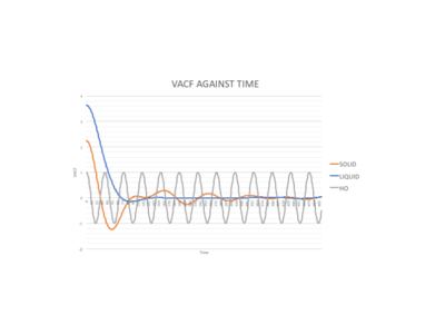
Figure 15 shows how VACF integrals for solid and liquid phases differ to the harmonic oscillator pathway. The VACF for the harmonic oscillator oscillates regularly between -1 and 1 due to the close packed regular structure of the approximation where there is no interatomic interaction. The graph shows that it has more long range ordering than the solid because it doesn't have to overcome any interatomic repulsions and that the liquid displays the least long range ordering. Neither of the phases coincide with the harmonic oscillator as it's far too regular and ideal.

Figure 16 Graph showing VACF vs. average time-step for solid phase

Figure 17 Graph showing VACF vs. average time-step for liquid phase

Figure 18 Graph showing VACF vs. average time-step for gas phase

		Diffusion Coefficients calculated using MSD data
		Solid	Liquid	Gas
	MSD	4.89E-05	0.090	4.92
	MSD 106 atoms	4.55E-05	8.33E-02	3.27

Once again, it can be seen that the diffusion coefficient increases from the solid to gaseous phase. Here the coefficient is calculated using velocities and so the higher diffusion coefficient corresponds to this increase in velocity. All three phases approach a maxima, and then the solid phase rise sharply down to 0 and fluctuates around this region. The fluctuation around 0 corresponds with the structured lattice of this phase, where the particles can only vibrate and have severely restricted movements. The liquid phase fluctuates around a value of 0.25. The gaseous phase however, does not reach fluctuation and the integral contrinues to increase expnenetially to the end of the averaging time-steps.

A big of error when estimating the diffusion coefficient from the VACF results from using the trapezium rule to approximate the integral under the VACF. The VACF graphs isn't strictly linear and more exponential-like, and hence the diffusion coefficient would be lower than expected when using this approximation. The error could be reduced by using a larger number of smaller trapeziums to calculate the integral, but this is a lot more extensive and may require more computing power. The trends obtained from the MSD and VACF methods align with one another and provide sufficient evidence that the three phases have been observed. The coefficients are within the same order for the liquid and gaseous phases, but not the solid phase. This may be due to statistical defects when simulating the positions of the particles in the MSD calculation, but most likely due to the error when using the trapezium rule in the VACF calculation.

Conclusion

In conclusion molecular dynamic simulations were used to examine the properties of the solid, liquid and vapour phases. The Lennard-Jones fluid was simulated in a NVE/NpT ensemble with varying timesteps and the thermodynamic properties were measured, such as heat capacity. The simulations were run under different temperatures, pressures, timesteps and densities. It was found that the optimal timestep was 0.0025 s in terms of computational efficiency and accuracy. Increasing the density of the system decreases with an increase in temperature and the heat capacity of a Lennard-Jones fluid decreases with increasing temperature, as well as with decreasing density. The RDF gave insight into the coordination numbers corresponding to the first three peaks for the solid phase and was determined from the integral of RDF graph. The diffusion coefficient then was calculated for the solid, liquid and gas via two different methods; MSD and VACF. The MSD was found to be a better method since there was a large source of error associated with the VACF method.