
Rep:Mod:Jake Hooton Physical Computational
Cope Rearrangement Tutorial
Antiperiplanar 1,5-hexadiene
A molecule of 1,5-hexadiene was built in Gaussview with an antiperiplanar conformation about the central C3-C4 bond. The molecular conformation was 'cleaned' using the clean tool from the edit menu and submitted for a Hartree-Fock 3-21G optimisation. The total energy of the optimised molecule was -231.69260235 a.u., as shown in the results summary below. Upon clicking 'symmetrize' in the edit menu, the results summary was no longer available, however the point group nomenclature of C1/C2 was indicated at the bottom of the viewing window.
Log file: Media:JH_COPE_OPT_HF321G.LOG
Results Summary:

Item Table:
Item Value Threshold Converged?
Maximum Force 0.000056 0.000450 YES
RMS Force 0.000010 0.000300 YES
Maximum Displacement 0.001457 0.001800 YES
RMS Displacement 0.000459 0.001200 YES
Predicted change in Energy=-2.090945D-08
Optimization completed.
-- Stationary point found.
Gauche 1,5-hexadiene
This time, a molecule of 1,5-hexadiene was built with a gauche conformation about the central C3-C4 bond. Again, the molecular conformation was 'cleaned' using the clean tool from the edit menu and submitted for a Hartree-Fock 3-21G optimisation. The total energy of the optimised molecule was -231.69153035 a.u., as shown in the results summary below. Again, upon clicking 'symmetrize' in the edit menu, the results summary was no longer available, however the point group nomenclature of C2/C1 was indicated at the bottom of the viewing window.
Log file: Media:JH_COPE_GAUCHE_OPT_HF321G.LOG
Results Summary:

Item Table:
 Item Value Threshold Converged?
Maximum Force 0.000035 0.000450 YES
RMS Force 0.000006 0.000300 YES
Maximum Displacement 0.000654 0.001800 YES
RMS Displacement 0.000183 0.001200 YES
Predicted change in Energy=-1.257929D-08
Optimization completed.
-- Stationary point found.
Comment/Results: The gauche conformation would be expected to be higher in energy than the antiperiplanar conformation, by analogy with the textbook case study of conformations about the central bond in butane - the app conformation is more stabilised due to higher E(2) energies of stabilisation, caused by the positioning of substituent groups around the bond in question. By comparing the total energies of the two conformations (this is possible because each calculation was run with the same method and basis set, and the molecules each have the same number of nuclei and electrons - they are simply conformational isomers of each other), it can be seen that the gauche confirmation is indeed 0.001072 a.u. higher in energy, or approximately 2.8 kJ mol-1.
By comparison with the provided table of the low energy conformations of 1,5-hexadiene in Appendix 1 of the instructions page, it can be observed that the optimised 'anti' structure of 1,5-hexadiene is the 'anti1' conformation, with C2 symmetry. The optimised 'gauche' structure of 1,5-hexadiene is the 'gauche4' structure, also with C2 symmetry. At first glance, it appeared that the 'anti1' and 'anti2' conformations were similar, however closer inspection revealed that the geometry of the double bonds about the central C3-C4 bond was different - the 'anti1' confirmation, to which my calculation had conformed, was slightly less symmetric, since it had each C-H unit (on carbon-2 and carbon-5 in the molecule) pointing on the same side of the molecule. Some small consideration led me to believe that the 'anti2' confirmation would be lower in energy, since it had each C-H unit (C2 and C5) pointing away on opposite sides of the molecule - giving it more symmetry and a marginally more linear structure. This would lead to less steric clash, more comfortable separation of nuclei and allowing better intermolecular stacking and dispersion forces in bulk amounts. For this reason, I next optimised 1,5-hexadiene to conform to the 'anti2' confirmation:
Finding the 'anti2' confirmation
The molecule was built to initially sit roughly in this conformation, and was then 'cleaned' and optimised by the same method to its ideal structure. Upon clicking 'symmetrize' when viewing the .chk file of the calculation results, the point group nomenclature of Ci/C1 was visible at the bottom of the viewing window (see thumbnail below), providing further evidence that the calculation had optimised to the correct conformation, since 'gauche3' is known to have Ci symmetry.
Log file: Media:JH_HEXADIENE_AIMFORCI_OPT_HF321G.LOG

Results Summary:

Item Table:
 Item Value Threshold Converged?
Maximum Force 0.000021 0.000450 YES
RMS Force 0.000006 0.000300 YES
Maximum Displacement 0.001299 0.001800 YES
RMS Displacement 0.000348 0.001200 YES
Predicted change in Energy=-2.283093D-08
Optimization completed.
-- Stationary point found.
Its total energy is observed to be -231.69253528 a.u. as shown in the results summary table. This is actually 0.00006707 a.u. higher in energy than the 'anti1' conformation, contrary to what I expected. However, these results do lie in agreement with those presented in Appendix 1 on the Instructions page, where 'anti2' has a total energy of -231.69254 a.u. (essentially the same value) and lies 0.00006 a.u. higher in energy than 'anti1'. Appendix 1 shows that 'gauche3' is actually the lowest energy conformation, with a total energy of -231.69266 a.u. The low energy of the 'gauche3' conformation can be rationalised by considering that each of the double bonds at the ends of 1.5-hexadiene have aligned themselves pointing away from each other, to reduce steric clash, and also favourably with the R group which comprises the rest of the molecule. This latter point of conformational analysis allows E2 stabilisations between the C4-H and C3-C4 bonds with the C5=C6 pi-cloud, and a favourable dispersion interaction between the remaining C4-H with one of the C6-H atoms.
More detailed optimisation of the 'anti2' conformation
The .chk file of the Hartree-Fock 3-21G optimisation of 'anti2' 3,5-hexadiene was submitted for a higher level calculation using the DFT method with B3LYP and a 6-31G* basis set, in order to compare the results, which are presented and discussed below.
Log file: Media:JH_HEXADIENE_ANTI2_OPT_DFT_631GD.LOG
Results Summary:

Item Table:
 Item Value Threshold Converged?
Maximum Force 0.000016 0.000450 YES
RMS Force 0.000007 0.000300 YES
Maximum Displacement 0.000263 0.001800 YES
RMS Displacement 0.000088 0.001200 YES
Predicted change in Energy=-1.674887D-08
Optimization completed.
-- Stationary point found.
The total energy is -234.61171035 a.u., a difference of -2.91917507 a.u. from the HF 3-21G optimisation, or approximately 7.6 x10³ kJ mol-1. This is a very large difference in energy and serves to demonstrate the higher level of accuracy and lower-energy optimisation results achieved using better basis sets such as 6-31G. Use of the inquisitor tool, to compare bond lengths from the two optimisations, reveals only very minor differences in the overall geometry between the two calculations on 1,5-hexadiene, therefore showing that slight adjustments in nuclear positions within a molecule lead to a large change in energy!
| HF 3-21G Optimisation | DFT 6-31G(d) Optimisation | ||||||
|---|---|---|---|---|---|---|---|
| C1=C2 | C2-C3 | C3-C4 | Molecule length C1-C6 | C1=C2 | C2-C3 | C3-C4 | Molecule length C1-C6 |
| 1.316 | 1.509 | 1.553 | 5.936 | 1.334 | 1.504 | 1.548 | 6.020 |
The main point to note is that the C=C double bonds are slightly longer (~0.02 Angstroms) in the DFT_6-31G(d) optimisation than in the HF_3-21G optimisation. The C-C single bond lengths are in contrast a tiny bit shorter in the DFT optimisation, but these changes are small by comparison (~0.005 Angstroms). These results also show that the DFT optimisation is found to be ~0.1 Angstroms longer across the whole molecule (C1 to C6 internuclear distance) than the HF optimisation. C-H bond lengths and all bond angles remain largely similar between the two optimised molecules, as do the bond lengths.
Frequency Calculations on the 'anti2' structure
The DFT_B3LYP_6-31G(d) optimised version of the 'anti2' conformation of 1,5-hexadiene, was submitted for a frequency calculation using the same method. The results are presented below:
Log file: Media:JH_HEXADIENE_ANTI2_FREQ_DFT_631GD.LOG
Results Summary:

Item Table:
Item Value Threshold Converged?
Maximum Force 0.000035 0.000450 YES
RMS Force 0.000014 0.000300 YES
Maximum Displacement 0.000291 0.001800 YES
RMS Displacement 0.000117 0.001200 YES
Predicted change in Energy=-1.590564D-08
Optimization completed.
-- Stationary point found.
Low Frequencies:
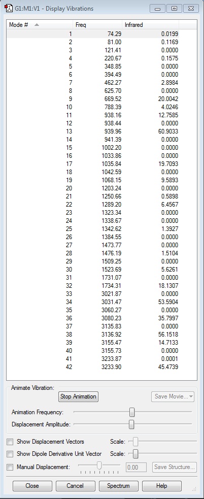
Low frequencies --- -9.4844 -0.0002 -0.0002 0.0004 3.7506 13.0164
Low frequencies --- 74.2861 80.9996 121.4176
The six low frequencies here are all equivalent to zero, bearing in mind that an accepted level of tolerance is within +/- 15 away from zero. This confirms that the optimisation has converged to a minimum and that there are no 'unreal' or negative frequencies, i.e. a transition state might have been found instead.
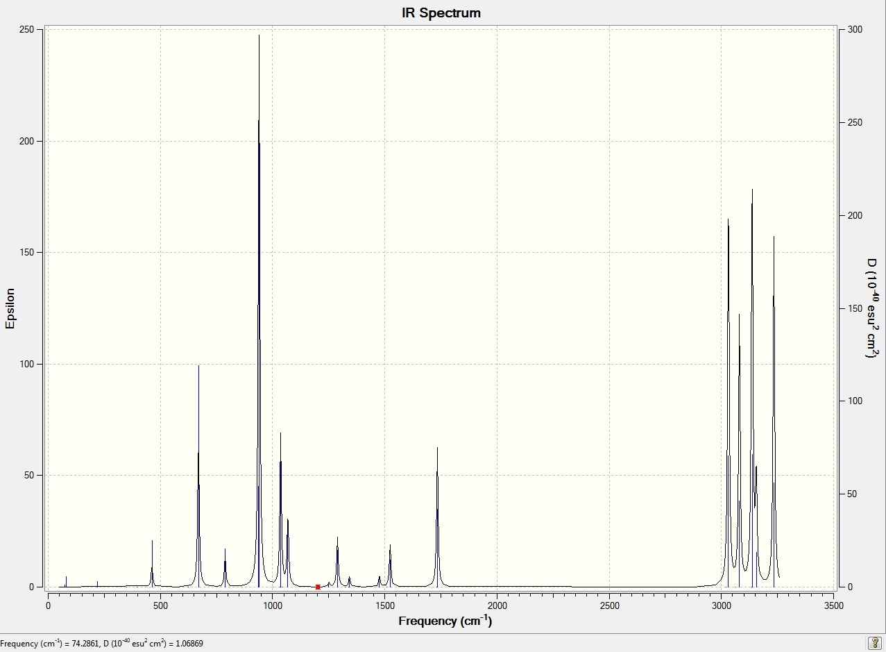
A full list of the computed frequencies may be found here: "Hexadiene Frequencies". All of these are real and positive too, meaning that there is not a problem. An animation of one of the frequencies is linked here: "Example Vibration" for display purposes, and the generated IR spectrum from this file is linked here: "JakeHooton_IR_spectrum_hexadiene.
Thermochemistry data:
Sum of electronic and zero-point Energies= -234.469204
Sum of electronic and thermal Energies= -234.461857
Sum of electronic and thermal Enthalpies= -234.460913
Sum of electronic and thermal Free Energies= -234.500777
Optimizing the "Chair" and "Boat" Transition Structures
Initial Fragment Optimisation
An allyl fragment was constructed in Gaussview and optimised at the HF/3-21G level of theory. The results are presented below:
Log file: Media:JAKEHOOTON_ALLYL_OPT_HF321G.LOG
Results Summary:

Item Table:
 Item Value Threshold Converged?
Maximum Force 0.000157 0.000450 YES
RMS Force 0.000036 0.000300 YES
Maximum Displacement 0.000636 0.001800 YES
RMS Displacement 0.000277 0.001200 YES
Predicted change in Energy=-7.608588D-08
Optimization completed.
-- Stationary point found.
First Method Transition State Calculation
The resulting structure was copied, and pasted twice to a new file, where the two fragments were manipulated to sit in a guessed position of the transition state. This required aligning the two fragments to sit in line with each other, in a 'chair' transition state, analogous to how a complete, six-membered cyclohexane ring would sit. By checking distances with the inquisitor tool, the internuclear distance between each pair of terminal carbons in the allyl fragments was adjusted to be 2.2 ± 0.03 Å.
The guessed structure was submitted for an Opt+Freq calculation, aiming for a Berny transition state, calculating the force constants once, at the HF/3-21G level with Opt=NoEigen to prevent the calculation from crashing. The results are presented below:
Log file: Media:JAKEHOOTON_OPTFREQ_TSBERNY_ONCE_NOEIGEN_HF321G.LOG
Results Summary:

Item Table:
 Item Value Threshold Converged?
Maximum Force 0.000033 0.000450 YES
RMS Force 0.000008 0.000300 YES
Maximum Displacement 0.001353 0.001800 YES
RMS Displacement 0.000370 0.001200 YES
Predicted change in Energy=-5.628890D-08
Optimization completed.
-- Stationary point found.
Low Frequencies:
Low frequencies --- -817.9334 -2.0605 -1.3173 -0.4888 0.0005 0.0006
Low frequencies --- 0.0008 209.5509 396.0369
****** 1 imaginary frequencies (negative Signs) ******
The calculation has successfully converged and it is indeed the same structure as the 'chair' transition state shown in Appendix 2 of the instructions page. The low frequencies results show that one negative (imaginary) frequency has been computed, confirming that a transition state has been found. The remaining frequencies are formally zero since a small tolerance about this point is accepted with low-level calculations. The negative frequency is -818 cm-1, in agreement with the value from the example calculation in the instructions page.
The vibration of frequency '-818 cm-1' is animated below.
| Animation of Vibration | Still picture showing Displacement Vectors for the Vibration |
|---|---|
| This vibration is indeed the transition state for the Cope Rearrangement. The animation on the left has dashed pi-bonds across the allyl fragments which alter as the fragments move (the dashed patterns change across the fragments, not just stretch with the bonds). This shows that the delocalisation of pi electrons across and between the allyl fragments is changing, and occupies space between and across the bonds in a cyclic transition state. These are criteria for a pericylic reaction, which is exactly what the Cope rearrangement is - a 3,3 sigmatropic rearrangement. The displacement vectors in the single-frame image on the right help to make clear the 3,3- nature of the rearrangement - the arrows on the right show two carbons moving 'outwards' from the ring, away from where the original sigma bond was, and the two arrows on the left show two carbons moving 'inwards' to close the gap, thus forming a new sigma bond on the opposite side of the ring. The ends of the new bond show a 3,3-relationship to the ends of the original sigma bond, which broke on the other side of the ring. | |
Second Method Transition State Calculation
The guess structure for the transition state, with terminal carbon internuclear distances of 2.2 Å, was again copied in to a new file. Using the redundant co-ordinates tool, the input file was edited so that the internuclear distances between terminal carbons was frozen. The structure was then optimised at the HF/3-21G level of theory, to minimise the fragments while not allowing the reaction to proceed. This optimised structure was then changed again with the redundant co-ordinates tool, this time so that the internuclear distances between terminal carbons were no longer fixed, but instead set to 'derivative'. This was to differentiate along the reaction co-ordinate in the following transition state optimisation, and obtain a good guess for the initial force constant matrix.
The new input structure was then submitted for a Opt+Freq calculation, again aiming for a Berny transition state, this time without calculating force constants. The keyword Opt=NoEigen was entered in order to prevent the calculation from crashing, and it was run at the HF/6-31G level of theory. The results are presented below:
Log File: Media:JAKEHOOTON_NEXTSTEP_SECONDTSCALC_MODREDUNDANT_HF321G.LOG
Results Summary:

Item Table:
 Item Value Threshold Converged?
Maximum Force 0.000112 0.000450 YES
RMS Force 0.000025 0.000300 YES
Maximum Displacement 0.001801 0.001800 NO
RMS Displacement 0.000488 0.001200 YES
Predicted change in Energy=-1.697675D-07
GradGradGradGradGradGradGradGradGradGradGradGradGradGradGradGradGradGrad
It can be seen from viewing the item table that the maximum displacement has not converged. However, upon talking to a demonstrator, I was told that I could in fact consider the calculation to have converged, since the numerical difference between the previous two iterations was so small that it had essentially converged. This was a very useful thing to learn since it meant I now realised the significance of these numbers and I could apply such reasoning myself.
Low Frequencies:
Low frequencies --- -817.8482 -0.8585 -0.0005 -0.0003 0.0005 4.8085
Low frequencies --- 6.9552 209.5595 395.9420
****** 1 imaginary frequencies (negative Signs) ******
The low frequencies table shows that with this method for finding the transition state, again just one negative frequency has been calculated. It is of magnitude 818 cm-1, in agreement with the first method which simply optimised to a transition state from the 'guessed' structure with the allyl fragments. Therefore, it can be considered to be the same vibration (the transition state) and it can be decided that both methods have worked.
A comparison of the structures from the two calculation methods is presented in the table below. Bond lengths were found by using the inquisitor tool.
| Force Constants Direct Optimisation from Guessed Structure | Frozen co-ordinates Method from Guessed Structure |
|---|---|
 |

|
| Top C...C internuclear distance: 2.02049 Å
Bottom C...C internuclear distance: 2.02028 Å C-C bond lengths: 1.38927 Å 1.38926 Å 1.38929 Å 1.38928 Å C-H bond lengths: 1.07599 Å 1.07585 Å 1.07599 Å 1.07424 Å 1.07424 Å |
Top C...C internuclear distance: 2.02035 Å Bottom C...C internuclear distance: 2.02082 Å
1.38932 Å 1.38926 Å 1.38932 Å 1.38926 Å C-H bond lengths: 1.07600 Å 1.07586 Å 1.07599 Å 1.07426 Å 1.07423 Å |
| It is obvious from the above data that the two transition states, found from different methods, are essentially identical. All corresponding bond lengths between the two structures are identical to three significant figures, and often to a higher degree of accuracy. | |
Optimising the Boat Transition Structure
In order to optimise the boat transition structure, an Opt+Freq calculation was used with the QST2 transition state method, instead of the Berny transition state method. This required setting up a file with multiple geometries. Namely, two of them - the reactant geometry and the product geometry. The optimised, Ci symmetry, 'anti2' structure of 1,5-hexadiene from earlier calculations was used in order to set this up. A new file was created with two geometries, and the 'anti2' structure copied in to each of them. Using the 'Atom List' editor, the numbering of the atoms in the carbon skeleton, with their corresponding hydrogens, was changed in the product geometry, in order to differentiate the product from the reactant and show that a rearrangement had taken place. It was important to make sure that the changes in atom numbering all consistently corresponded with the original positions of the atoms in the reactant geometry.
Th calculation was set to run finding a QST2 transition state (no force constants calculations or keywords), however the calculation fails because the initial structures were not even close to a well-guessed transition state. Upon editing the reactant and product structures to better resemble the boat transition state (by using the bond angle and bond dihedral angle tools to change the geometry about C2-C3-C4-C5 for the reactant and product structures), the calculation was repeated and this time it converged to a transition state without a problem. The results are presented below:
Log File: Media:JAKEHOOTON_OPTANDFREQ_SECOND_QST2_BOATALIGNED_FORCECONSTANTSNEVER_NOKEYWORDS_HF321G.LOG
Checkpoint File: Media:JakeHooton_OptAndFreq_Second_QST2_BoatAligned_ForceConstantsNever_NoKeywords_HF321G.chk
Results Summary:

Item Table:
 Item Value Threshold Converged?
Maximum Force 0.000095 0.000450 YES
RMS Force 0.000025 0.000300 YES
Maximum Displacement 0.001233 0.001800 YES
RMS Displacement 0.000401 0.001200 YES
Predicted change in Energy=-2.718081D-07
Optimization completed.
-- Stationary point found.
Low Frequencies:
Full mass-weighted force constant matrix:
Low frequencies --- -840.2308 -1.5389 0.0005 0.0007 0.0008 4.2802
Low frequencies --- 7.9268 155.3833 382.0899
****** 1 imaginary frequencies (negative Signs) ******
It is clear from the low frequencies table that there is only one imaginary frequency, this time of magnitude 840 cm-1, different to the chair transition structure. This vibration (showing the transition state) is animated in the table below.
| Frequency Table | Animated Vibration (Log File) | Displacement Vectors | Checkpoint File Picture |
|---|---|---|---|
 The imaginary frequency is at the top of the table here. The imaginary frequency is at the top of the table here. |
 Please click on the file to view the animation, for some reason it does not work when it is embedded here! Please click on the file to view the animation, for some reason it does not work when it is embedded here! |
 The displacement vectors show that a sigmatropic shift is occurring - two terminal carbons are moving away from each other, while the other two are moving towards each other. The displacement vectors show that a sigmatropic shift is occurring - two terminal carbons are moving away from each other, while the other two are moving towards each other. |
Predicting Product Conformations with the Intrinsic Reaction Co-ordinate
From observing the chair and boat transition structures calculated above, it is difficult to tell which product conformation they will lead to. In order to work this out, an intrinsic reaction co-ordinate (IRC) calculation was carried out, using the first optimised chair transition state as an example (a direct optimisation from a guessed transition state, not the frozen co-ords or QST2 method). Since, for the Cope Rearrangement, the IRC is symmetrical backwards and forwards, the calculation was chosen to only calculate forwards, since it would give the same result. Force constants were chosen to be calculated always, and 50 iterations were chosen in the hope that the product conformation would converge.
It was found eventually that the output file had stopped after 44 iterations. Further instruction to better optimise the molecule suggested running a standard optimisation from the final iteration, running the IRC again with more steps, or choosing to calculate the force constants at every step. Since the latter of these methods had been employed in the first place, both of the former two methods were used. The standard HF/3-21G optimisation led to a slight change in structure, whereas running the IRC from the start with 80 steps led to exactly the same result - the iterations stopped after no. 44 and the structure was identical to the IRC calculation with 50 steps. This led me to believe that the IRC had in fact converged to a good result. The product geometry from the chair transition state was identified as the 'gauche2' conformation of 1,5-hexadiene by comparison with Appendix 1. The results for each calculation are presented below:
| Initial IRC, 50 steps | HF/3-21G Optimisation of final iteration from 50-step IRC | Extra IRC, 80 steps |
|---|---|---|
| Log file: Media:JHIRCCALC.LOG | Log file: Media:NORMALOPTAFTER.LOG | Log file: Media:JHIRCCALCMORE.LOG |
Animation:  |
 |

|
| This output structure can be considered fully optimised by any of the above three methods.
As mentioned before, it is consistent with the 'gauche2' conformation of 1,5-hexadiene, when comparing with Appendix 1. | ||
Higher Level Optimisations to compare and find the activation energy
In order to compare activation energies for the Cope Rearrangement proceeding via each transition state, the total energies of each structure must be compared between the reagent, the chair transition state, and the boat transition state. They must all be optimised at the same level to make the comparison meaningful, and a higher level basis set must be used in order to give more accurate energies. Therefore, the chair transition state from the 'best guess - direct optimisation' (first) method, and the boat transition state from the calculations in part e), were re-optimised to a Berny Transition State at the DFT/6-31G(d) level. The results and a comparison are presented below:
N.B. - The earlier IRC calculation confirmed, at least with the chair transition state, that the rearrangement proceeds via this transition state, between the 'gauche2' conformations of 1,5-hexadiene. Ideally, when comparing the total energy of the optimised transition states with the reactant, they should be compared with the correct conformer of the reactant from which they proceed in a cope rearrangement. However, the differences in energy between different conformations of the reactant is small compared with the activation energy from the reaction. Therefore, both the chair TS and the boat TS are compared directly with the 'anti2' conformer of 1,5-hexadiene below, in light of a lack of time to run extra (working!) IRC calculations on the boat TS and extra optimisations on other conformers of 1,5-hexadiene. This can be justified because the quantitative error is small, and broad comparisons of the activation energy for each transition state can be easily made with the 'anti2' conformer. This is sufficient for what we would like to achieve at the moment.
| Reactant | Chair TS | Boat TS |
|---|---|---|
| Log file: Media:JH_HEXADIENE_ANTI2_OPT_DFT_631GD.LOG | Log File: Media:JakeHootonCHAIRTS_DFT.LOG | Log file:Media:JakeHootonBOATTS_DFT.LOG |
Picure:  |
Picture:  |
Picture: 
|
Item Table: Item Value Threshold Converged? Maximum Force 0.000016 0.000450 YES RMS Force 0.000007 0.000300 YES Maximum Displacement 0.000263 0.001800 YES RMS Displacement 0.000088 0.001200 YES Predicted change in Energy=-1.674887D-08 Optimization completed. -- Stationary point found. |
Item Table: Item Value Threshold Converged? Maximum Force 0.000022 0.000450 YES RMS Force 0.000005 0.000300 YES Maximum Displacement 0.000079 0.001800 YES RMS Displacement 0.000025 0.001200 YES Predicted change in Energy=-3.728079D-09 Optimization completed. -- Stationary point found. |
Item Table: Item Value Threshold Converged? Maximum Force 0.000009 0.000450 YES RMS Force 0.000003 0.000300 YES Maximum Displacement 0.000144 0.001800 YES RMS Displacement 0.000052 0.001200 YES Predicted change in Energy=-2.675669D-09 Optimization completed. -- Stationary point found. |
Low Frequencies
Low frequencies

-9.4844 -0.0002
-0.0002 0.0004
3.7506 13.0164

Low frequencies --- 74.2861 80.9996
121.4176
No negative frequencies |
Low Frequencies Low frequencies -565.5417 -0.0006 -0.0002 0.0006 21.9498 27.2872 Low frequencies --- 39.7423 194.5207 267.9554 1 imaginary frequencies (negative Signs) |
Low Frequencies Low frequencies -530.3620 -8.4026 -0.0007 0.0005 0.0011 15.4606 Low frequencies --- 17.6111 135.6112 261.7009 1 imaginary frequencies (negative Signs) |
| Total Energy -234.61171035 a.u. | Total Energy -234.55698303 a.u. | Total Energy -234.54309307 a.u. |
| The difference in total energy between the 'anti2' reactant and the chair transition state is +0.05472732 a.u. or 144 kJ mol-1. The difference in total energy between the 'anti2' reactant and the boat transition state is +0.06861728 or 180 kJ mol-1. | ||
Comment/Discussion: The difference in total energy between the 'anti2' reactant and the chair transition state is +0.05472732 a.u. or 144 kJ mol-1. The difference in total energy between the 'anti2' reactant and the boat transition state is +0.06861728 or 180 kJ mol-1. Therefore, it can be concluded that the chair transition state is preferable for the cope rearrangement. 36 kJ mol-1 is a large difference in activation energy in terms of chemical kinetics, therefore it can also be concluded that the reaction will almost never proceed via the boat transition state, since the chair transition state is so much more preferable. Comparisons can easily be drawn between this reasoning and the famous case-study of conformational analysis with cyclohexane, the definitive six-membered ring. Cyclohexane's lowest energy conformation is the chair conformation, and its boat conformation actually represents a local energy maximum, converting between the two twist-boat local minima. These in turn are higher in energy than the chair conformation, providing results which back up the conclusion from these transition state calculations.
Diels-Alder Transition States
A structure of cis-butadiene was constructed in gaussview and submitted for an optimisation with the semi-empirical AM1 method, in order to initially gain some idea about the structure of its MOs. The results are presented below:
Log file: File:JAKEHOOTON CISBUTADIENEMO.LOG
| HOMO | LUMO |
|---|---|
 |
 |
| The HOMO is antisymmetric (a) with respect to reflection about the plane of symmetry bisecting the molecule. Green lobes are mapped on to red lobes, and vice versa. | The LUMO is symmetric (s) with respect to reflection about the plane of symmetry bisecting the molecule. The terminal red and green lobes are mapped on to their counterparts at the other end of the molecule. Each half of the central red lobe and the central green lobe is mapped on to the other half of that lobe, when reflected about this plane of symmetry. |
The same thing was then done for ethene:
Log file: Media:JHOOTONETHENE_AM1.LOG
| HOMO | LUMO |
|---|---|
 |
 |
| The HOMO on ethene is symmetric (s) with respect to reflection about the plane of symmetry bisecting the molecule. Each half of the green lobe and the red lobe is mapped on to the other half of that lobe, when reflected about this plane of symmetry. | With ethene, the LUMO is antisymmetric (a) with respect to reflection about the plane of symmetry bisecting the molecule. Red lobes are mapped on to green lobes, and vice versa, when reflected over this plane of symmetry, and a change of phase is observed with this mapping. |
Optimising the Diels-Alder Transition State
Failed QST2 Method
Many methods were tried in order to optimise the Diels-Alder transition state, including the QST2 method, the direct optimisation from a guess method, and the optimisation with frozen co-ordinates method. Eventually, only the direct guess method provided the correct transition state. An account of how these calculations were run is presented below:
Initially, a QST2 method was prepared This required first optimising separate molecules of butadiene, ethene, and cyclohexene with a semi-empirical AM1 basis set, of which the results are presented here (in the form of log files): Butadiene, Ethene, Cyclohexene.

The butadiene and ethene molecules were appended in to the same window and the structure was edited such that their position represented a feasible approach for the reaction to take place. By reference to this paper, http://pubs.acs.org/doi/pdf/10.1021/ja01036a004, the C3-C4 and C5-C6 bond lengths in cyclohexene were noted to be 1.515 ± 0.020 Å. Therefore, for the initial approach geometry, I set the internuclear distance between the terminal, bond-forming C...C atoms in each fragment to be slightly larger, at 1.8 Å, as can be seen in the thumbnail on the right, highlighted with the inquisitor tool. The optimised cyclohexene was placed in the next frame, and the numbering of each atom in the initial and final states was checked in order to make sure that they correctly corresponded. The input structure is presented as an image file with the thumbnail on the right. The calculation was optimised with a QST2 method, but unfortunately it failed.
The filed output is presented as a log file here: QST2 Calculation
In order to improve this calculation, I decided a QST3 calculation, with a guessed transition structure also in the input, might be more successful. However, if I was to guess the transition structure, I decided the direct guess or frozen co-ordinates methods might be more successful.
Successful Direct Guess Method
Again, for this calculation, I used the reactant structures which I had pre-optimised with the semi-empirical AM1 basis set. I appended the butadiene and ethene in to the same file and adjusted them so that they had a reasonable approach trajectory. At this point I asked the demonstrator about whether it was necessary to change the bonds to dashed bonds for a guessed transition state. He told me it would not make any difference, since Gaussian only read the positions of the atoms, but that I should try a slightly larger internuclear distance between the terminal C...C atoms, of the order of 2.2 Å. I set the terminal carbon internuclear distances to 2.15 Å, and proceeded with an optimisation to a Berny Transition state. In this case the calculation failed since the molecules were too far apart, and Gaussian was trying to optimise them as separate molecules side by side. The output file terminated after 100 steps.
Log file of failed direct guess: Media:JHOOTONDIRECTGUESSDA_AM1.LOG
Animation of Failed Optimisation to a Berny TS:

I proceeded to run another 'Direct-Guess', Opt+Freq calculation to a Berny transition state, this time with shorter terminal carbon internuclear distances of 1.70 Å. This calculation successfully obtained the transition state, the results are presented below.
Log file of Successful TS Opt+Freq: Media:JHOOTONDIRECT2.LOG

Final, failed attempt with the frozen co-ordinates method
For the purposes of comparison, I also attempted to find this transition state with the frozen co-ordinates method. I copied my previous, guessed approach geometry (from the previous direct-guess calculation) to a new file. Terminal carbon internuclear distances were still 1.7 Angstroms. This time, I optimised the structure initially with the terminal internuclear distances frozen. At this point, the calculation worked well, everything converged (in the item table), and I was ready to continue to the next step.
Log file of initial optimisation: Media:JHOOTONPREOPT_AM1.LOG
Next, similarly to the method in the training exercise, I changed the internuclear carbon distances from being frozen, to 'derivative'. The new input file was submitted for an Opt+Freq calculation to a Berny TS, never calculating force constants, with the semi-empirical AM1 basis set and the keyword Opt=NoEigen. This calculation did complete successfully, however upon checking the outputted log file, the results were not correct:
Log file: Media:JHOOTONMODREDTSOPT_AM1.LOG
In the item table below, it can be seen that the maximum displacement has not converged for the structure in this calculation.
Item Table:
 Item Value Threshold Converged?
Maximum Force 0.000074 0.000450 YES
RMS Force 0.000011 0.000300 YES
Maximum Displacement 0.002968 0.001800 NO
RMS Displacement 0.000802 0.001200 YES
Predicted change in Energy=-6.866716D-09
In the low frequencies table below this, it can be seen that the one negative frequency corresponding to the transition state, only has a magnitude of 53 cm-1. This rang alarm bells, since it was much too low.
Low Frequencies:
Low frequencies --- -52.6225 -4.8214 -3.5450 -3.0324 -0.0026 0.0160
Low frequencies --- 0.1893 152.2198 380.7794
****** 1 imaginary frequencies (negative Signs) ******
Indeed, animating the transition state vibration (see below), showed that it was wrong. This vibration does not correspond to forming new C-C bonds, instead it just shows a bending vibration for two methylene units in the ring:


Further Analysis with Correct Transition State
The 'Direct-Guess' method was the only one which provided the correct transition state, therefore it was considered for further analysis and discussion. The log file is provided again below:
Log file: Media:JHOOTONDIRECT2.LOG
Item Table:
Item Value Threshold Converged?
Maximum Force 0.000064 0.000450 YES
RMS Force 0.000012 0.000300 YES
Maximum Displacement 0.000923 0.001800 YES
RMS Displacement 0.000262 0.001200 YES
Predicted change in Energy=-1.025422D-07
Optimization completed.
-- Stationary point found.
Low Frequencies:
Low frequencies --- -956.2947 -3.0249 -0.0480 -0.0062 -0.0030 2.6671
Low frequencies --- 3.8191 147.3572 246.6003
****** 1 imaginary frequencies (negative Signs) ******
Transition State Vibration:
There is one negative frequency here, of magnitude 956 cm-1. This confirms that the transition state has been found correctly. the motion of this vibration is animated below, and again it can be seen that this is indeed the correct motion for the transition state in question:


From observing the above animation on the right, it can be seen that the formation of the two new sigma bonds between the pairs of terminal carbon atoms is synchronous, or concerted. Both bonds definitely form at the same time, not one before the other. This observation agrees with the general theory of pericyclic reactions - they proceed via a cyclic transition state with concerted movement of electrons. From an arrow-pushing point of view, there is no 'correct' direction. The arrows can be pushed in either direction, therefore no bond could really be expected to form before the other one - the reaction happens in one step.
First Positive Vibration:
The synchronous, transition state oscillation animated above is contrasted strongly by the oscillation for the first positive vibration for this optimised transition state. The first positive vibration oscillates in an asynchronous manner, as shown in the animation below:


HOMO and LUMO of the transition State:
The HOMO and LUMO of this transition state are presented below:
| HOMO | LUMO |
|---|---|
 |
 |
| The HOMO on the transition state is antisymmetric (a) with respect to reflection about the plane of symmetry bisecting the structure, by observing the change in phase of the orbital lobes in this operation. | The LUMO of the transition state is symmetric (s) with respect to reflection about the plane of symmetry bisecting the structure, this time by observing the lack of change in phase of the orbital lobes in this operation. |
The HOMO of the transition state corresponds to the interaction between the HOMO of butadiene and the LUMO of ethene, each of which are antisymmetric as mentioned above, which correspond to the antisymmetric nature of the transition state HOMO.
The LUMO of the transition state, on the other hand, corresponds to the interaction between the LUMO of butadiene and the HOMO of ethene, each of which are symmetric in nature, and correspond to the symmetric nature of the transition state LUMO.
In a reaction, the electrons still occupy the lowest energy orbitals of the transition state, therefore the electrons involved in the reaction are those in the HOMO. Thus, it can be concluded that the reaction proceeds from the HOMO of butadiene and the LUMO of ethene. This makes sense, since in Diels-Alder reaction is is typically the diene that is electron rich and the dieneophile which is electron poor. The rare, alternate cases are known as 'Reverse Electron Demand Diels-Alder reactions'.
The reaction itself is allowed to proceed because these orbitals share the same symmetry label (displayed earlier) and they can overlap efficiently, allowing the movement of electrons and the reaction to occur.
Exo and Endo: Cyclohexadiene with Maleic Anhydride Diels-Alder Transition State
Initially, molecules of cyclohexadiene and maleic anhydride were optimised with the semi empirical AM1 basis set, in order to provide template files from which to find the transition state. The log files are presented below:
Cyclohexadiene: Media:JHOOTON_CYCLOHEXADIENEOPT.LOG
Maleic Anhydride: Media:JHOOTON_MALANHYDRIDEOPT.LOG
To locate transition states for this Diels-Alder reaction, I decided straight away to employ the frozen-coordinates method. The optimised cyclohexadiene and maleic anhydride were both appended to the same input file, and orientated as follows. This optimisation was set up to aim for the stabilised, endo transition state. The pi-system of maleic anhydride (extended across its two carbonyl functionalities and the oxygen atom between them) is angled so that it sits above the pi-system of cyclohexadiene, rather than pointing in the opposite direction over the sigma-framework. In this way, it can stabilise the pi-system of cyclohexadiene during the transition state in this Diels-Alder reaction. The terminal carbon internuclear distances (between the pairs of carbon atoms forming sigma bonds in this reaction) were set to 1.72 Å, as a reasonable guess for the initial approach trajectory. This structure was optimised to a minimum with the semi-empirical AM1 basis set, with the terminal internuclear C...C distances frozen.
Log File: Media:JHOOTON_PREMODREDUND.LOG


As can be seen above in the animation on the right, this calculation proceeded without error and produced a structure leading towards the endo- transition state. This could be further optimised to the actual transition state in the next step.
Unfortunately this step failed. Instead, the Exo and Endo transition states were found by employing a QST3 method:
Using the QST3 Method
Initially, molecules of each reactant were and product were optimised with the semi-empirical AM1 basis set. The log files are presented here: Cyclohexadiene, Maleic Anhydride, Endo Product, Exo Product.
These were appended to a QST3 input file. The reactant molecules were aligned suitably for the endo and exo approach trajectory in each case, the product geometries were already optimised, and the guessed transition states (3rd window) were in each case copied from a frozen co-ordinates optimisation of the transition state in question (endo or exo) with the terminal C...C bond forming pairs frozen. The freezing of these atoms was removed completely for the QST3 calculations, the atom numbering was made consistent through each geometry in the endo and the exo case, and the QST3 calculations were submitted. Force constants were calculated 'once', and the semi-empirical AM! basis set was used.
N.B.- In each case, the approach trajectories had internuclear C...C distances of approx 2.15 Angstroms, the transition state internuclear C...C distances were inputted having before been frozen at about 1.7 Angstroms, and the C-C bond lengths in the product had been pre-optimised at the level of the semi-empirical AM1 basis set, and were equal to about 1.55 Angstroms. In each case, the calculations were successful and led to the correct transition state. The results are presented below and the transition state vibrations are animated:
Endo:
Input File:

Output Log File: Media:JHOOTON_ENDO_QST3.LOG
Results:

Please view the vibration here: Media:JHooton_Success_QST3_Endo.gif
Exo:
Input File:

Output Log file: Media:JHOOTON_EXO_QST3.LOG
Results:


Note/Comment: The exo form is more strained, because it is not stabilised by a pi-overlap effect from the pi-system on maleic anhydride, and also it suffers from steric clash where the oxygen atoms on maleic anhydride clash with methylene hydrogens on the other fragment.