Rep:Mod:JPS1124
Third Year CMP Compulsory Experiment James Simpson (CID:00733493)
Introduction to the Ising Model
The Model
| Number of Dimensions | Number of Neighbors |
|---|---|
| 1 | 2 |
| 2 | 4 |
| 3 | 6 |
| D | 2D |
The Ising model is an physics model used in order to understand the behaviour of ferromagnets. Ferromagnets are materials in which the magnetic dipoles of the material align so that an overall magnetic dipole is exhibited by the material. This effect is due to the favourable energy minimisation due to the alignment of the dipoles or spins. However this will unfavourably decrease the entropy. In the model only spins between neighbouring lattice points interact. This interaction is defined as , where J is a constant and si and sj are the spins of the lattice point and its neighbour. The third rule is that a cell at the edge of the lattice will interact with another cell at the other edge of the lattice; this is so that all possible neighbours will be interacted with. The number of neighbours in a particular number of dimensions is expressed in table 1.
The interaction energy of a number of particles in a particular number of dimensions can be expressed as . This can be shown using the initial equation in the lab script of . From table 1 it is clear that the number of neighbours each lattice cell has is equal to twice the number of dimensions. The first step is to show what the lowest interaction energy must be; in the lowest energy all the magnetic spins are parallel and so this means that the term in the equation will simply be equal to the number of neighbours which is 2-D. This is simply done N times as there as N number of particles and so . This is then multiplied by the constant of , giving the interaction energy to be . From this point it is possible to consider the multiplicity of the system. Ordinarily in chemistry the multiplicity of a system is given by the equation , but this cannot be done in this case as the values of the magnetic spin are integers and so the lattice cells can be considered as quasi-boson particles. As the equation stated in the previous sentence is designed for electrons it must be ignored, as in the case of a one-lattice cell unit it would give a multiplicity of 3 where a value of 2 is logically expected. All the magnetic spins in a ferromagnetic material will be aligned so that the spins are all parallel, however the spins of each lattice cell can have a value of +1 or a value of -1. This means that the number of micro-states is 2 and so the multiplicity is 2. It then follows that the entropy of the system given by , where Ω is the number of micro-states, in this case the multiplicity of the system. Therefore the entropy of the system is simply which is 9.570x10⁻²⁴ JK-1.
Phase Transition
In the lowest energy configuration the interaction energy is -3000J. However, when one spin changes the interaction energy of the system will naturally increase. In order to consider how much the energy increases when a spin flips, the effect this will have on the system must be thought about. It is equivalent to removing the spin entirely and putting back into the system another spin, but with a direction opposite to the rest of the system. When a spin is removed the system will lose six interactions, one for each neighbour, and then when the opposite spin is added there will be six interactions created: however this will increase the interaction energy by 6J. So, the flipping of the spin destabilizes the energy by 12J in total as 6J of favourable interactions are lost and 6J of unfavourable interactions are gained. This leads to the interaction energy of this system being -2988J. The new entropy of the system will be as the new spin can occur anywhere in the lattice and there are 1000 options for that, and in addition there will be 2 options for every point in the lattice where the opposite spin will be. This is because the majority of the system can a have a spin of +1, where the opposite spin will be -1. The other option is where most of the system will have a spin of -1 and in this case the opposite spin will have a value of +1. This means when compared to the lowest energy configuration the entropy will have increased by , which is 9.54x10⁻²³ JK-1.

The Curie temperature is the temperature below which ferromagnetism will be exhibited. At temperatures below the Curie temperature the stabilisation energy will be large enough to compensate for the loss in entropy. However above the Curie temperature this is not the case and the entropy effect will dominate, leading to the material showing diamagnetism. Magnetisation is given as and so in all cases the magnetisation is simply the difference between the number of +1 spins and the number of -1 spins. In the case of the 1-D lattice there are three +1 spins and two -1 spins and so the magnetisation will be simply +1. For the 2-D case there are thirteen +1 spins and twelve -1 spins, meaning that the magnetisation again in that case is +1. Although both of the systems in figure 1 are not very magnetised, the Ising lattice in 3-D containing 1000 lattice cells at absolute zero will be highly magnetised. As the system is at absolute zero there will be no thermal energy available in order to overcome the spin flipping energy barriers, therefore it is expected that the system will adopt the lowest energy configuration, which is where all the spins align. This means that the value of the magnetisation will be equal to the number of lattice cells, in this case 1000. Therefore the magnetisation is either -1000 or +1000, but it cannot be known which of these two options is correct without further investigation.
Calculating the Energy and Magnetisation
Whenever the ipython programme was loaded the following two lines were run in order to start the session %load_ext autoreload and %autoreload 2. Firstly the files IsingLattice.py and ILcheck.py were extracted and stored in the H:Drive.
Modifying the Files
This section involved two parts: one of these was to find the magnetisation while the other was to find the energy of a random arrangement of a specific lattice size, determined by the user. The code used to find the magnetisation is shown below:
   def magnetisation(self):
       magnetisation = 0
       for i in range(self.n_rows):
           for j in range (self.n_cols):
               magnetisation += self.lattice [i,j]
       #Return the total magnetisation of the current lattice configuration.
       return magnetisation
The code used to determine the energy of the lattice is shown below:
   def energy(self):
       ener = 0.0
       for i in range(self.n_rows):
           for j in range (self.n_cols):
           # 1st row, 1st column corner
               if j == 0:
           # Last row, 1st column corner
                   if i == self.n_rows-1:
                       ener += self.lattice [i,j]*self.lattice [0,j]
                       ener += self.lattice [i,j]*self.lattice [i,j+1]
           # Rest of 1st column
                   else:
                       ener += self.lattice [i,j]*self.lattice [i+1,j]
                       ener += self.lattice [i,j]*self.lattice [i,j+1]
           # 1st row, last column corner
               elif j == self.n_cols-1:
           # Last row, last column corner
                   if i == self.n_rows-1:
                       ener += self.lattice [i,j]*self.lattice [0,j]
                       ener += self.lattice [i,j]*self.lattice [i,0]
           # Rest of last column
                   else:
                       ener += self.lattice [i,j]*self.lattice [i+1,j]
                       ener += self.lattice [i,j]*self.lattice [i,0]
               else:
           # Rest of last column
                   if i == self.n_rows-1:
                       ener += self.lattice [i,j]*self.lattice [0,j]
                       ener += self.lattice [i,j]*self.lattice [i,j+1]
           # Rest of lattice
                   else:
                       ener += self.lattice [i,j]*self.lattice [i+1,j]
                       ener += self.lattice [i,j]*self.lattice [i,j+1]
       energy = ener*-1
       "Return the total energy of the current lattice configuration."
       return energy
Testing the Code
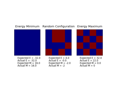
This code was then tested using the file Ilcheck.py which created three lattices and checked the energy and magnetisation of these lattices. One configuration corresponded to the energy minimum, one to the energy maximum, and one to an random intermediate state: this was found to work as expected. The result of this and a checkpoint, while that did not work as expected, are shown below.
 |
 |
|---|---|
| Figure 2: A Incorrect Checkpoint File | Figure 3: The Correct Checkpoint File |
Introduction to the Monte Carlo simulation
Average Energy and Magnetisation
A system that contains 100 lattice cells with each lattice cell being allowed to be one of two states, spin up or spin down, has a certain number of states available to it. Using the equation for the number of micro-states , where n is the number of energy levels available and N is the number of particles, it is found that the number of micro-states will be or 1.27x1030 states. If the computer can analyse 109 configurations in a second then it would take 1.27x10²¹ seconds to analyse all the configurations. As this number is too large to be meaningful it has been converted to years, and in years it would take 4.02x10¹³ years to analyse all the configurations, longer than the age of the universe!
Importance Sampling.
The code used for the Monte Carlo simulation is shown below:
   def montecarlostep(self, T):
       # complete this function so that it performs a single Monte Carlo step
       energy = self.energy()
       magnetisation = self.magnetisation()
       #the following two lines will select the coordinates of the random spin for you
       random_i = np.random.choice(range(0, self.n_rows))
       random_j = np.random.choice(range(0, self.n_cols))
       #the following line will choose a random number in the rang e[0,1) for you
       random_number = np.random.random()
       # Randomly change a spin
       if self.lattice [random_i, random_j] == 1:
       # From 1 go to -1
           self.lattice [random_i, random_j] = -1
       else:
       # From -1 go to 1
           self.lattice [random_i, random_j] = 1
       energy1 = self.energy()
       magnetisation1 = self.magnetisation()
       deltaenergy = energy1 - energy
       if deltaenergy < 0:
       # Energy goes down
           energy = energy1
           magnetisation = magnetisation1
       elif random_number <= exp(- deltaenergy/ T):
       # Energy goes up but smaller than random number
           energy = energy1
           magnetisation = magnetisation1
       else:
       # Energy goes up and larger than random number
           self.lattice [random_i, random_j] = - self.lattice [random_i, random_j]
       self.E += energy
       self.E2 += energy**2
       self.M += magnetisation
       self.M2 += magnetisation**2
       self.n_cycles += 1
       return energy, magnetisation
   def statistics(self):
       # complete this function so that it calculates the correct values for the averages of E, E*E (E2), M, M*M (M2), and returns them
       aveE = self.E/self.n_cycles
       aveE2 = self.E2/self.n_cycles
       aveM = self.M/self.n_cycles
       aveM2 = self.M2/self.n_cycles
       return aveE, aveE2, aveM, aveM2
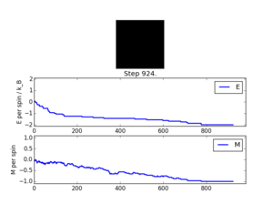
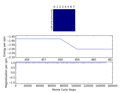
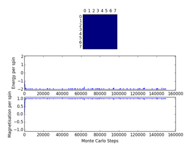
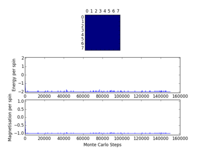
The code was then tested using the file ILanim.py; this ran a Monte Carlo simulation of an eight by eight lattice and displayed the output at a temperature of 1 temperature unit. The results of two runs of this testing, including the display output, can be seen opposite. In one case all the spins in the system became +1, while in the other case the spins in the system became -1. As has been stated earlier, below the Curie temperature the lattice will be ferromagnetic and so the spins will align. This means that it is expected that there will be spontaneous magnetisation.
Accelerating the Code
In order to check if the code has been accelerated it was necessary to check how quick the original code was, as an accelerated code must be quicker. The speed of the original code was tested using the file ILtimetrial.py, which ran 2000 steps of the Monte Carlo simulation. This was done 5 times and then averaged, as each time it ran there were slightly different timings. The times of each run and the average can be seen from table 4 below.
| Attempt 1 | Attempt 2 | Attempt 3 | Attempt 4 | Attempt 5 | Average Time Taken |
|---|---|---|---|---|---|
| 6.5321323358111965 | 6.5576305262353145 | 6.548430656233478 | 6.566359750713659 | 6.561720323517164 | 6.553254719 |
The standard error of the sample was found to be 0.006049722. Using the numpy.sum function, a new code for the magnetisation was made. This code is shown below:
def magnetisation(self):
       magnetisation = np.sum(self.lattice)
       return magnetisation
The new code for determining the energy is show below. This was done using the numpy multiply and numpy roll functions.
   def energy(self):
       np.multiply(self.lattice, np.roll(self.lattice,1,axis=0))
       np.multiply(self.lattice, np.roll(self.lattice,1,axis=1))
       return energy
The code still gave the expected result when tested using the file ILcheck.py, this can be seen to the below:

The file ILtimetrial was used again in order to find how long the new code would take to perform 2000 Monte Carlo steps. As can be seen below, the new code was much faster than the original, 0.387094820036961 seconds compared to 6.553254719 seconds. The standard error was also decreased, 0.000177801 compared to 0.006049722. This means that the new code worked more quickly than the original and was more consistent in the time taken to perform 2000 Monte Carlo steps.
| Attempt 1 | Attempt 2 | Attempt 3 | Attempt 4 | Attempt 5 | Average Time Taken |
|---|---|---|---|---|---|
| 0.384887314998096 | 0.38467463684389713 | 0.3845507255513354 | 0.3855771603227396 | 0.3848634022924955 | 0.387094820036961 |
The Effect of Temperature
Correcting the Averaging Code
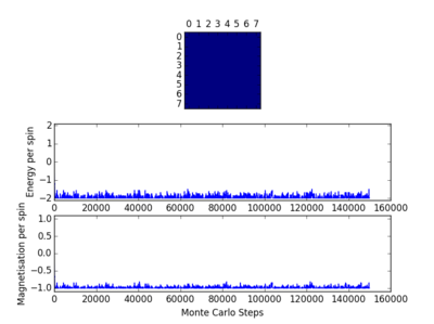
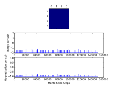
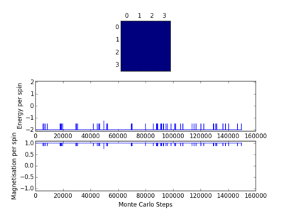
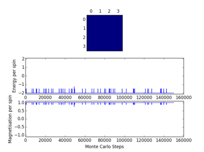
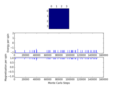
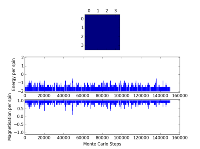
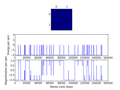
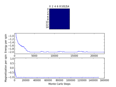
The behaviour of the lattice using the Ising model can now be tested in order to probe further into the Curie temperature, the area where the change of domination between the enthalpic and entropic terms takes place. As it takes time for the system to reach the equilibrium state this will affect the outcome of any experiment taking place, so it will be necessary to ignore the first few Monte Carlo steps until the equilibrium state is reached; as has been seen earlier, the energy sharply decreased before the minimum energy was reached. The energy and magnetisation should only be averaged after equilibrium has been reached. Lattices of different sizes and different temperature had 150000 Monte Carlo steps performed on them using the file Il.finalframe.py and the number of steps required to reach equilibrium are shown below.
As can be seen from table 6, the amount of time required for the energy to be minimised varied depending on a number of factors, the temperature of the system and the size of the lattice. Decreasing the number of lattice points from an 8x8 lattice to a 4x4 lattice, a decrease of 75%, resulted, on average, in the number of Monte Carlo steps needed for the energy to be minimised being decreased by a factor of 10. The number of Monte Carlo steps needed when the temperature was increased from 1 to 1.5 is not shown. The reason for this is clear if the diagrams within table 6 are examined: at a higher temperature more high level energy levels will be populated and so the minimum energy will be less easily observed, indeed has not been observed in either the 8x8 or 4x4 lattice at 1.5. The number of Monte Carlo steps needed was also different in each run as can be seen from table 6. It is better to overestimate the number of steps that will be required than to underestimate. All the values of Monte Carlo steps required for a 4x4 lattice were less than 100 and for a 8x8 lattice they were all less than 1000: therefore the first 100 steps should be ignored for a 4x4 lattice and the first 1000 steps should be ignored for an 8x8 lattice. The file ILfinalframe.py was then modified with the following addition and alterations - a new variable was made n_ignore, which was the number of Monte Carlo steps that were to be ignored.
       if self.n_cycles >= self.n_ignore:
           self.E += energy
           self.E2 += energy**2
           self.M += magnetisation
           self.M2 += magnetisation**2
           self.n_cycles += 1
       else:
           pass
       return energy, magnetisation

   def statistics(self):
       # complete this function so that it calculates the correct values for the averages of E, E*E (E2), M, M*M (M2), and returns them
       aveE = self.E/(self.n_cycles-self.n_ignore)
       aveE2 = self.E2/(self.n_cycles-self.n_ignore)
       aveM = self.M/(self.n_cycles-self.n_ignore)
       aveM2 = self.M2/(self.n_cycles-self.n_ignore)
       return aveE, aveE2, aveM, aveM2, self.n_cycles
This code was altered so that, if the count was below the number of Monte Carlo steps needed before the lattice that reached the minimum energy, then the energy and magnetisation were not added to. The second change was that the average energy, energy squared, magnetisation and magnetisation squared were altered so that they only averaged for the number of counts that they had had added. In table 7. it is possible to see the number of ignored Monte Carlo steps for different size lattice.
Running Over a Range of Temperatures
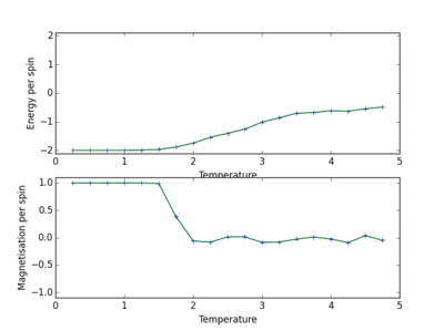
The following code was changed in the file IsingLattice.py and the empty lists El and Ml were made:
   def statistics(self):
       # complete this function so that it calculates the correct values for the averages of E, E*E (E2), M, M*M (M2), and returns them
       aveE = self.E/(self.n_cycles-self.n_ignore)
       aveE2 = self.E2/(self.n_cycles-self.n_ignore)
       aveM = self.M/(self.n_cycles-self.n_ignore)
       aveM2 = self.M2/(self.n_cycles-self.n_ignore)
       sdeve = np.std(self.El)
       sdevm = np.std(self.Ml)
       serre = sdeve / sqrt(self.n_cycles-self.n_ignore)
       serrm = sdevm / sqrt(self.n_cycles-self.n_ignore)
       return aveE, aveE2, aveM, aveM2, self.n_cycles, serre, serrm
From the file ILtemperaturerange.py the code was changed to:
   from IsingLattice import *
   from matplotlib import pylab as pl
   import numpy as np
   n_rows = 4
   n_cols = 4
   n_ignore = 100
   il = IsingLattice(n_rows, n_cols)
   il.lattice = np.ones((n_rows, n_cols))
   spins = n_rows*n_cols
   runtime = 10000
   times = range(runtime)
   temps = np.arange(0.25, 5.0, 0.25)
   energies = []
   magnetisations = []
   energysq = []
   magnetisationsq = []
   serrma = []
   serren = []
   for t in temps:
       for i in times:
           if i % 100 == 0:
               print(t, i)
           energy, magnetisation = il.montecarlostep(t)
       aveE, aveE2, aveM, aveM2, n_cycles, serre, serrm = il.statistics()
       energies.append(aveE)
       energysq.append(aveE2)
       magnetisations.append(aveM)
       magnetisationsq.append(aveM2)
       serrma.append(serrm)
       serren.append(serre)
       #reset the IL object for the next cycle
       il.E = 0.0
       il.E2 = 0.0
       il.M = 0.0
       il.M2 = 0.0
       il.n_cycles = 0
   fig = pl.figure()
   enerax = fig.add_subplot(2,1,1)
   enerax.set_ylabel("Energy per spin")
   enerax.set_xlabel("Temperature")
   enerax.errorbar(temps, np.array(energies)/spins, xerr=0, yerr= np.array(serren)/spins)
   enerax.set_ylim([-2.1, 2.1])
   magax = fig.add_subplot(2,1,2)
   magax.set_ylabel("Magnetisation per spin")
   magax.set_xlabel("Temperature")
   magax.errorbar(temps, np.array(magnetisations)/spins, xerr=0, yerr= np.array(serrma)/spins)
   magax.set_ylim([-1.1, 1.1])
   enerax.plot(temps, np.array(energies)/spins)
   magax.plot(temps, np.array(magnetisations)/spins)
   pl.show()
   final_data = np.column_stack((temps, energies, energysq, magnetisations, magnetisationsq))
   np.savetxt("8x8.dat", final_data)
 |
 |
|---|---|
| 8x8 | 4x4 |
The Effect of System Size
From the previous section the energies and spins of different lattice sizes at different temperatures were found so that the onset of phase transition could be seen. It is possible to show all the data sets on the same graph and by doing this the minimum lattice size needed to accurately model the long range fluctuations that occur within the system. The code used in order to do this is shown below:
   def temp(file):
       data = np.loadtxt(file)
       temp = data[:,0]
       return temp

   def energy(file):
       filenum = int(file.split('x')[0])
       num = filenum*filenum
       data = np.loadtxt(file)
       energ = data[:,1]
       energy = energ/num
       return energy

   def magn(file):
       filenum = int(file.split('x')[0])
       num = filenum*filenum
       data = np.loadtxt(file)
       mag = data[:,3]
       magn = mag/num
       return magn

   def plot(a,b,c,d,e):
       fig = pl.figure()
       enerax = fig.add_subplot(2,1,1)
       enerax.set_ylabel("Energy per spin")
       enerax.set_xlabel("Temperature")
       enerax.set_ylim([-2.1, 0])
       magax = fig.add_subplot(2,1,2)
       magax.set_ylabel("Magnetisation per spin")
       magax.set_xlabel("Temperature")
       magax.set_ylim([-1.1, 1.1])
       enerax.plot(temp(a), energy(a),temp(b), energy(b),temp(c), energy(c),temp(d), energy(d),temp(e), energy(e))
       enerax.legend(["2x2", "4x4", "8x8", "16x16", "32x32"],bbox_to_anchor=(0., 1.02, 1., .102), loc=3,ncol=5, mode="expand", borderaxespad=0.)
       magax.plot(temp(a), magn(a),temp(b), magn(b),temp(c), magn(c),temp(d), magn(d),temp(e), magn(e))
       pl.legend()
   pl.show()
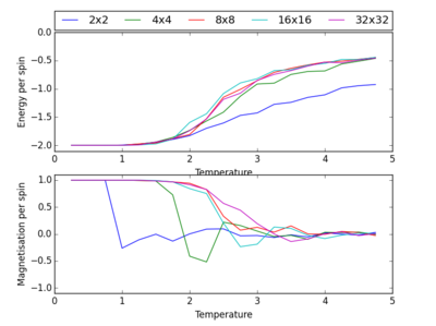
The graph made by this code is shown on figure 24, to the right and it is clear that an 8x8 lattice is the minimum size necessary to observe the long term fluctuations. From the energy part of the graph the energies are almost the same from an 8x8 lattice and larger and so it is pointless to compute for a larger lattice as it will not improve the results.
Determining the Heat Capacity
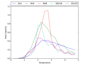
Increasing the temperature above the Curie temperature induces a phase transition. This means that the magnetisation of the system will rapidly drop and from this the heat capacity of the system can be found using the relationship . It is known that the heat capacity should become very strongly peaked at the phase transition temperature and the code used to plot a graph showing the heat capacity versus temperature for each of lattice size is:
   def temp(file):
       data = np.loadtxt(file)
       temp = data[:,0]
       return temp

   def temp2(file):
       data = np.loadtxt(file)
       temp = data[:,0]
       temp2 = temp*temp
       return temp2

   def energy(file):
       filenum = int(file.split('x')[0])
       num = filenum*filenum
       data = np.loadtxt(file)
       energy = data[:,1]
       return energy

   def energy2(file):
       filenum = int(file.split('x')[0])
       num = filenum*filenum
       data = np.loadtxt(file)
       energy2 = data[:,2]
       return energy2

   def var(file):
       var = energy2(file) - (energy(file)*energy(file))
       return var

   def heat(file):
       filenum = int(file.split('x')[0])
       num = filenum*filenum
       heat = (var(file)/temp2(file))/num
       return heat

   def plot(a,b,c,d,e):
       fig = pl.figure()
       pl.ylabel("Heat Capacity")
       pl.xlabel("Temperature")
       pl.ylim([0, 1.2])
       pl.plot(temp(a), heat(a),temp(b), heat(b),temp(c), heat(c),temp(d), heat(d),temp(e), heat(e))
       pl.legend(["2x2", "4x4", "8x8", "16x16", "32x32"],bbox_to_anchor=(0., 1.02, 1., .102), loc=3,ncol=5, mode="expand", borderaxespad=0.)
       pl.legend()
       pl.show()
The result of this code can be seen below:
Locating the Curie Temperature
Comparison of Python Data with C++ Data
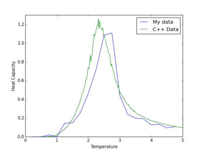
It is clear from the previous section that the heat capacity becomes strongly peaked in the vicinity of the critical temperature around 2 to 2.5. The peak of the heat capacity became more sharp as the lattice size was increased. If there was an infinite size lattice then the critical temperature would diverge at the Curie temperature. Obviously this is not possible and in fact, not only does the heat capacity not diverge with different lattice sizes but the Curie temperature also changes. However the temperature at which the maximum heat capacity is found is modeled using the equation , TC,L is the Curie temperature of an LxL lattice and TC, inf is the Curie temperature of an infinity large lattice; A is a constant which is not important. It is possible to compare a C++ program, that has run much longer simulations, to the data computed using Python. The code used for this is shown below and the comparison for an 8x8 lattice is shown to the right:
   def temp(file):
       data = np.loadtxt(file)
       temp = data[:,0]
       return temp

   def temp2(file):
       data = np.loadtxt(file)
       temp = data[:,0]
       temp2 = temp*temp
       return temp2

   def energy(file):
       filenum = int(file.split('x')[0])
       num = filenum*filenum
       data = np.loadtxt(file)
       energy = data[:,1]
       return energy

   def energy2(file):
       filenum = int(file.split('x')[0])
       num = filenum*filenum
       data = np.loadtxt(file)
       energy2 = data[:,2]
       return energy2

   def energy2(file):
       filenum = int(file.split('x')[0])
       num = filenum*filenum
       data = np.loadtxt(file)
       energy2 = data[:,2]
       return energy2

   def var(file):
       var = energy2(file) - (energy(file)*energy(file))
       return var

   def heat(file):
       filenum = int(file.split('x')[0])
       num = filenum*filenum
       heat = (var(file)/temp2(file))/num
       return heat

   def cap(file):
       data = np.loadtxt(file)
       cap = data[:,5]
       return cap

   def plot(a,b):
       fig = pl.figure()
       pl.ylabel("Heat Capacity")
       pl.xlabel("Temperature")
       pl.ylim([0, 1.3])
       pl.plot(temp(a), heat(a),temp(b), cap(b))
       pl.legend(["My data", "C++ Data"])
       pl.legend()
       pl.show()
Polynomial fitting
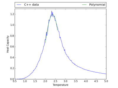
In order to find where the heat capacity is at a maximum, the data will be fitted to a polynomial. This is done using the polyfit and polyval functions from NumPy. The result of this can be seen below with a 11th order polynomial fit along with the code used.
   def plot(file):
       data = np.loadtxt(file) #assume data is now a 2D array containing two columns, T and C
       T = data[:,0] #get the first column
       C = data[:,5] # get the last column
       fit = np.polyfit(T, C, 101) # fit a third order polynomial
       T_min = np.min(T)
       T_max = np.max(T)
       T_range = np.linspace(T_min, T_max, 1000) #generate 1000 evenly spaced points between T_min and T_max
       fitted_C_values = np.polyval(fit, T_range) # use the fit object to generate the corresponding values of C
       pl.ylabel("Heat Capacity")
       pl.xlabel("Temperature")
       pl.ylim([0, 1.3])
       pl.plot(T, C, T_range, fitted_C_values)
       pl.legend(["C++ data", "Polynomial"])
       pl.show()

Fitting in a particular temperature range
This code could then be modified so that it only fitted the data in the region required. The polynomial used to fit the data was a 3rd order one. The change is shown below:
   def plot(file):
       data = np.loadtxt(file) #assume data is now a 2D array containing two columns, T and C
       T = data[:,0] #get the first column
       C = data[:,5] # get the last column
       T_min = 2.0
       T_max = 2.6
       T_range = np.linspace(T_min, T_max, 1000) #generate 1000 evenly spaced points between T_min and T_max
       selection = np.logical_and(T > T_min, T < T_max) #choose only those rows where both conditions are true
       peak_T_values = T[selection]
       peak_C_values = C[selection]
       fit = np.polyfit(peak_T_values, peak_C_values, 3)
       fitted_C_values = np.polyval(fit, T_range) # use the fit object to generate the corresponding values of C
       pl.ylabel("Heat Capacity")
       pl.xlabel("Temperature")
       pl.ylim([0, 1.3])
       pl.plot(T, C, T_range, fitted_C_values)
       pl.legend(["C++ data", "Polynomial"], bbox_to_anchor=(0., 1.02, 1., .102), loc=3,ncol=5, mode="expand", borderaxespad=0.)
       pl.show()
Finding the peak in C
| Lattice Size | Tmax | Cmax |
|---|---|---|
| 2x2 | 2.52252252 | 0.414795316278 |
| 4x4 | 2.45345345 | 0.816615090356 |
| 8x8 | 2.36276276 | 1.19327965652 |
| 16x16 | 2.31931932 | 1.56571895874 |
| 32x32 | 2.29479479 | 1.83746564575 |
The code was then altered in order to find the maximum values of the heat capacity, and the temperature this occurred at, for different lattice sizes: from this the Curie temperature could be found. The values of Tmax and Cmax for the different size lattices can be seen on the right in table 8 (for 2x2, 4x4, and 8x8 a 3rd order polynomial was just, for a 16x16 a 5th order polynomial was used and for the 32x32 lattice a 7th order polynomial was used). The result from changing the code can be seen result below:
   def plot(file):
       data = np.loadtxt(file) #assume data is now a 2D array containing two columns, T and C
       T = data[:,0] #get the first column
       C = data[:,5] # get the last column
       T_min = 2.0
       T_max = 2.5
       T_range = np.linspace(T_min, T_max, 1000) #generate 1000 evenly spaced points between T_min and T_max
       selection = np.logical_and(T > T_min, T < T_max) #choose only those rows where both conditions are true
       peak_T_values = T[selection]
       peak_C_values = C[selection]
       fit = np.polyfit(peak_T_values, peak_C_values, 7)
       fitted_C_values = np.polyval(fit, T_range) # use the fit object to generate the corresponding values of C
       Cmax = np.max(fitted_C_values)
       Tmax = T_range[fitted_C_values == Cmax]
       pl.ylabel("Heat Capacity")
       pl.xlabel("Temperature")
       pl.ylim([0, 2])
       pl.plot(T, C, T_range, fitted_C_values)
       pl.legend(["C++ data", "Polynomial"], bbox_to_anchor=(0., 1.02, 1., .102), loc=3,ncol=5, mode="expand", borderaxespad=0.)
       pl.show()
       print (Cmax)
       print (Tmax)
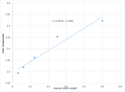
These results could be ploted using the equation , this was done on Microsoft Excel for simplicity and this can be seen from figure 29. The equation of the trend-line of this data is also shown and gives the value of to be 2.2962. This compares quite well to a literature value of of 2.2691. This could be improved by using a higher order polynomial in order to more accurately find Cmax and therefore more accurately find Cinf.
Reference
1. J. Kotze, Introduction to Monte Carlo methods for an Ising Model of a Ferromagnet, http://arxiv.org/pdf/0803.0217.pdf

