
Rep:Mod:Ifv611
Part 1: Familiarisation with Inorganic Computational Techniques
Introduction
This module aimed to investigate physical properties, and in particular the structure and bonding modes, of compounds by modeling them and using Gaussian to run optimisations and analyses based on it. The tasks assigned for the first week were intended to be used to get comfortable with using Gaussian, GaussView and the HPC SCAN portal to run optimisations, frequency analyses and population analyses. All the optimisation methods fall within the DFT (density functional theory) category, i.e. use functions or combinations of multiple functions to predict the ground state structure of specific molecules.
Optimisation of BH3
Optimising a molecule of BH3
After creating the BH3 on Gaussview 5.0 and breaking its symmetry by setting the BH bond lengths as respectively 1.53 Å, 1.54 Å and 1.55 Å, an optimisation calculation was set up to be run on Gaussian 09 using the DFT-B3LYP method and the 3-21G basis set. The optimisation file is linked to here, and its summary can be seen in Figure 1.

The logbook entry, showing convergence, is:
Item               Value     Threshold  Converged?
 Maximum Force            0.000038     0.000450     YES
 RMS     Force            0.000020     0.000300     YES
 Maximum Displacement     0.000266     0.001800     YES
 RMS     Displacement     0.000156     0.001200     YES
 Predicted change in Energy=-9.722686D-09
 Optimization completed.
    -- Stationary point found.
                           ----------------------------
                           !   Optimized Parameters   !
                           ! (Angstroms and Degrees)  !
 --------------------------                            --------------------------
 ! Name  Definition              Value          Derivative Info.                !
 --------------------------------------------------------------------------------
 ! R1    R(1,2)                  1.1944         -DE/DX =    0.0                 !
 ! R2    R(1,3)                  1.1943         -DE/DX =    0.0                 !
 ! R3    R(1,4)                  1.1943         -DE/DX =    0.0                 !
 ! A1    A(2,1,3)              120.0239         -DE/DX =    0.0                 !
 ! A2    A(2,1,4)              119.9735         -DE/DX =    0.0                 !
 ! A3    A(3,1,4)              120.0026         -DE/DX =    0.0                 !
 ! D1    D(2,1,4,3)            180.0            -DE/DX =    0.0                 !
 --------------------------------------------------------------------------------
In addition to showing convergence, the portion of the *.log file copied above also shows that the value of the derivative of the forces on all atoms and bonds is indeed zero. This table of Optimised Parameters will be considered implicit from now on and omitted (although it can always be found in the output file, which will always be included).
This optimised molecule had bond lengths and angles that were not exactly identical (as one would expect in a symmetrical trigonal planar molecule). The bond distances calculated were: 1.19436 (B-H2), 1.19433 (B-H3) and 1.19434 (B-H4), which when taking into consideration the 0.01 Å accuracy of the calculation is the same as saying that they were all equal to 1.19 Å; while the angles were found to be: 120.024 (H2-B-H3), 120.003 (H3-B-H4) and 119.974 (H4-B-H2). These bond lengths coincide with the reference value of 1.190 01(1) Å [1], while the bond angles have a maximum deviation of 0.026° from the 120° predicted by VSEPR theory.
Understanding Optimisation

Using Gaussview, the Gaussian output file *.log can also be opened to show all intermediate Geometries, i.e. the series of iterative structures modeled by Gaussian in the search for an equilibrium structure. This particular display mode also allows us to examine quantitatively the numerical values of the first derivative for each step by producing two equivalent optimisation plots, seen in Figure 2. They are closely related to each other, in the sense that while the Total Energy plot gives the exact values for the energy of the correspondent intermediate geometry, the RMS Gradient plot depicts the forces acting on each intermediate structure. Although describing the behavior of the first derivative function, the gradient plot is actually a weighted average of such derivative across the three degrees of freedom given by the possible displacements in space of each BH bond. The whole optimisation process aims to reduces these forces to zero, to ensure the modelling of the minimum energy structure. This structure is the one in which all atoms are at in their equilibrium position. Although this process tends to reduce the energy with every step, knowing that the forces on a specific structure are zero does not necessarily prove that we are in presence of a minimum energy structure. Since such forces are given by the first derivative of the energy as a function of the atoms' coordinates, any stationary point would render such function null, but it still has to be proven which type of stationary point we are dealing with in this case (maximum or minimum). It is interesting to note that a Transition State structure would correspond to a maximum in energy and therefore its gradient would also be zero. This is where the frequency analysis (that involves performing the second derivative of the energy as a function of the atoms' positions) comes useful (see later).
We can see that as expected the gradient average at the optimised structure is zero, and that the energy is reduced to the value that then appears in the summary (Figure 1).
This view mode also allows to navigate through intermediate geometries, and see what structures Gaussian proposes for each of these. It might be worth nothing that a few of this proposed structures do not have bonds drawn in and as such might appear slightly confusing. This only means that that specific optimisation step contains inter-atom distances that are larger than Gaussian's definition of a maximum bond length (which is probably close to the sum of the Van der Waal's radii of the two atoms). While this is just a technicality, it is quite hard to define exactly what makes a bond a bond and what is just interactions within nonbonded atoms. What is certain is that a real bond is most definitely not a line joining two atoms, although this is the most convenient and widely recognised way of drawing one. As IUPAC defines it[2], a bond is an interaction within atoms with strength sufficient to lead to a complex stable enough to be considered as an independent molecular species. Since the interactions between B and H atoms considered here are obviously leading to the formation of our BH3 molecule, we can safely assume that Gaussian should indeed have drawn some bonds.
Using a better basis set
The first rough optimisation done can serve as a starting point for a better one with a larger and more complex basis set. While the method is still B3LYP the basis set used is now 6-31G(d,p). The *.log file for this calculation can be found here. A summary is shown in Figure 3 and the logbook entry showing convergence follows.

  Item               Value     Threshold  Converged?
 Maximum Force            0.000018     0.000450     YES
 RMS     Force            0.000011     0.000300     YES
 Maximum Displacement     0.000090     0.001800     YES
 RMS     Displacement     0.000060     0.001200     YES
 Predicted change in Energy=-2.343925D-09
 Optimization completed.
    -- Stationary point found.
The optimised bond lengths and distances give us a proof (albeit a weak one since the accuracy of values cannot be trusted with such small percentage differences) that using a larger basis set gets us closer to the empirical values of these properties. In fact this time the calculated bond lengths are only about 0.00230 Å larger than the reference ones[1] and the angles only present a maximum deviation of 0.013° from the expected values. These numbers are a much better indicator of the relative effectiveness of a specific basis set since they don't depend on it; in contrast the two optimised energies of BH3 (respectively -26.46226427 AU and -26.61532361 AU for the two successive optimisations) cannot be compared as they are strictly relative to the functions contained in the basis set used.
Optimisation of GaBr3
After creating this molecule on Gaussview 5.0, the optimization was set up on Gaussian to be executed with the B3LYP method and using the LanL2DZ basis set, i.e. a hybrid method involving the use of specific basis sets for lighter atoms and pseudo-potentials for the heavier ones. The calculation was performed on the HPC SCAN portal (DOI:10042/27614 ).
The symmetry of this molecule had to be forced to D3h through the Point Group menu on Gaussian to avoid future problems. This explains why the two previously modeled molecules are classified as having a lower symmetry than expected (Cs rather than D3h) while for this molecule Gaussian is able to pick up the higher symmetry level.
A summary of the optimisation can be seen in Figure 4 and the logbook entry showing convergence follows.

	Item               Value     Threshold  Converged?
 Maximum Force            0.000000     0.000450     YES
 RMS     Force            0.000000     0.000300     YES
 Maximum Displacement     0.000003     0.001800     YES
 RMS     Displacement     0.000002     0.001200     YES
 Predicted change in Energy=-1.282685D-12
 Optimization completed.
    -- Stationary point found.
The optimised bond lengths and were found to be particularly close to empirical value, with all Ga-Br bonds presenting the same lenght (2.35018 Å, coinciding with the reference value of 2.3525 Å [3]) and all Br-Ga-Br angles being 120°, as predicted by VSEPR.
Optimisation of BBr3
This calculation was setup by changing the H atoms in the 6-31G(d,p) optimised BH3 file into Br atoms and then performing a hybrid pseudo-potentials/basis set optimisation on this molecule within the HPC SCAN portal. The method used this time was GEN, which allows to set specific basis sets for each atom, with the additional pseudo=read gfinput keywords, allowing to also set a specific basis set for each atom and to specify which one by editing the input file with Notepad or similar text editor (unfortunately the editing cannot be done within Gaussview). It was chosen to use a combination of the 6-31G(d,p) basis set and the LanL2DZ pseudo potential.
This calculation was performed by the HPC SCAN portal (DOI:10042/27617 ); a summary of the optimisation can be seen in Figure 5 and the logbook entry showing convergence follows.

Item               Value     Threshold  Converged?
 Maximum Force            0.000022     0.000450     YES
 RMS     Force            0.000012     0.000300     YES
 Maximum Displacement     0.000115     0.001800     YES
 RMS     Displacement     0.000072     0.001200     YES
 Predicted change in Energy=-2.437083D-09
 Optimization completed.
    -- Stationary point found.
By using the inquire function on Gaussview the B-Br optimised bond lengths were found to be larger than the reference value of 1.900(4) Å measured through Gas phase diffraction [4]. The bond lengths reported in the output file were in fact equal to 1.93 Å. It might be interesting to note that the overestimation of BBr3 bond lengths by DFT basis sets has already been reported by the literature[5] and therefore the search for a bigger or better basis set might not be useful in reaching a better optimisation as it looks like its an intrinsic error of this particular computational method.
The bond angles reported were very close to the ideal 120° angle predicted by VSEPR, presenting a maximum deviation of only 0.005° from this value.
Comparison of BH3, GaBr3 and BBr3 Bond lengths
| BH3 | BBr3 | GaBr3 |
|---|---|---|
| 1.19232 Å (lit. value: 1.1900 Å [1]) | 1.93396 Å (lit. value: 1.9000 Å [4]) | 2.35018 Å (lit. value: 1.3525 Å[3]) |
Since all these molecules have the same trigonal planar structure with D3h point group, we can compare their respective bond lengths to investigate the effects of central atoms and ligands on bond lengths. The molecules that have been investigated conveniently can be picked in groups of two to analyse either variation (central atom or ligand).
The effect of ligand change can be seen in the difference between BH3 and BBr3 bond lengths. In fact, the presence of Br increases the bond length by about 60% (a little more if considering the computed values). This can be rationalised by remembering that it is substantially larger and heavier than hydrogen. Therefore we can conclude that the larger atomic radius of bromine (related to its position in the third row of the periodic table and its ability to populate p and d-orbitals) is a dominating factor in determining bond length. Another factor to consider is the difference in electronegativity between the atoms forming the bonds: Δχ is larger for the B-Br couple rather than for the B-H couple. Such difference implies a greater mismatch between orbital energies and therefore a poorer overlap, resulting in a weaker and hence longer bonds. Additionally it might be worth noting that we would expect the B-H bond to be rather covalent in character and the B-Br bond to be more ionic.
The other axis of comparison can be investigated by comparing BBr3 and GaBr3. The latter was found to be about 22% larger than the former, as could be expected since Gallium is larger than Boron. Another factor is the quality of orbital overlap between the ligand and the central atom: the 4p orbitals available for bonding in Gallium are more diffuse compared to the 2p orbitals available to Boron, and therefore do not overlap as well. A better orbital overlap leads to stronger and therefore shorter bonds, matching the observed bond lengths. The higher electronegativity difference between Gallium and Bromine when compared with the B-Br couple is further reason for a worse orbital overlap, since as mentioned before it implies orbital energies being further apart.
Frequency Analysis for BH3
As mentioned previously, the gradient of the PES does not give any indication regarding which type stationary point has our ensemble of functions converged towards. To ensure we are in the presence of a ground state molecule and not a Transition state we have to take the second derivative of the PES and check that its value is positive. This is essentially what the Frequency analysis comprises, in addition to being able to predict IR and Raman spectra for computed molecules.
The frequency calculation was run on Gaussian from the 6-31G(d,p) optimised BH3 molecule. The complete analysis can be found (as *.log file) here, a summary can be seen in Figure 6 and the logbook entry showing convergence follows.

Item               Value     Threshold  Converged?
 Maximum Force            0.000029     0.000450     YES
 RMS     Force            0.000011     0.000300     YES
 Maximum Displacement     0.000179     0.001800     YES
 RMS     Displacement     0.000085     0.001200     YES
 Predicted change in Energy=-4.155592D-09
 Optimization completed.
    -- Stationary point found.
Unfortunately the analysis of the low frequencies did not yield the expected results: although the "real" frequencies have the expected values, the low "near zero" frequencies, representing the motions of the molecule about the center of motion, are actually not near zero enough. They are reported here:
 Low frequencies ---  -24.2753  -11.0052   -0.0006   -0.0002   -0.0001   14.0575
 Low frequencies --- 1162.9993 1213.0431 1213.1899
Observation of the summary shows that the molecule has been optimised with point group Cs and this low symmetry level could be a reason for such strong "near zero" frequencies.
To investigate this further, it was decided to add the opt=tight, scf=conver=9 and int=ultrafine keywords to the optimisation in order to force the symmetry to D3h and to start the frequency analysis again.
The output of this second frequency analysis can be found here, its summary is shown in Figure 7 and the logbook entry showing convergence follows.

Item               Value     Threshold  Converged?
 Maximum Force            0.000004     0.000450     YES
 RMS     Force            0.000002     0.000300     YES
 Maximum Displacement     0.000017     0.001800     YES
 RMS     Displacement     0.000008     0.001200     YES
 Predicted change in Energy=-1.087480D-10
 Optimization completed.
    -- Stationary point found.
Now the analysis of low frequencies gives the expected results: much lower "near zero" frequencies and reasonable frequencies.
 Low frequencies ---  -11.7227  -11.7148   -6.6070    0.0008    0.0278    0.4278
 Low frequencies --- 1162.9743 1213.1388 1213.1390
Opening the frequency analysis output file on Gaussview allows us to visualize the vibrational modes, summarized in Table 2. As expected for a non-linear molecule, BH3 has vibrational modes (i.e. 6 modes since BH3 has 4 atoms).
| No. | Form of Vibration | Frequency [cm-1] | Intensity | Symmetry D3h point group | No. | Form of Vibration | Frequency [cm-1] | Intensity | Symmetry D3h point group |
|---|---|---|---|---|---|---|---|---|---|
| 1 |  |
1162.97 | 95.5682 | A2" | 4 |  |
2582.58 | 0.00 | A1' |
| The 3 H atoms move in and out of the plane following the arrows, B follows the same movement but in opposite phase. This corresponds to the out-of-plane (ν2) normal mode of vibration, or "wagging". | All the H atoms move in and out together in the same plane following the arrows shown, B stays stationary. This is a totally symmetric stretching vibrational mode (ν1), also called "breathing". | ||||||||
| 2 |  |
1213.14 | 14.0550 | E' | 5 |  |
2715.72 | 126.3320 | E' |
| The 3 H atoms move on the same plane. H(2) and H(3) move towards each other, H(4) and H(3) move away from each other, making H(4) and H(2) have the same movement in the same direction, B balances the movement. This "rocking" motion is one of the two degenerate vibrational modes corresponding to the asymmetric stretching (ν3) normal mode. | H(2) and H(4) move in and out along their respective B-H bond alternatively. The boron atom and H(3) balance. the movement. This is one of the two degenerate in-plane bending (ν4) normal vibrational modes. | ||||||||
| 3 |  |
1213.14 | 14.0544 | E' | 6 |  |
2715.72 | 126.3260 | E' |
| H(2) and H(4) move towards each other following the arrows shown, the B atom balances the movement by moving along the B-H(3). This is the other degenerate ν3 "scissoring" (bending) vibrational mode. | H(2) and H(4) move together along their respective B-H bond, while H(3) follows a similar movement along its B-H bond, but out of phase with respect to the other two. B balances the movement of H(3). This is the second degenerate ν4 symmetrical stretching vibrational mode. |

Although the atoms are not numbered in the pictures within Table 7. all the snippets have been taken while the molecule was in the same orientation: the H molecule at the top is referred to in the vibrational descriptions as H(3), the next one going clockwise is H(2) and the last one is H(4).
The frequency calculation performed by Gaussian also allows Gaussview to display a prediction for the IR spectrum of BH3, such spectrum can be seen in Figure 8.
It is worthy of note that although the Gaussian output file showed 6 vibrations, we can only observe 3 vibrations in the predicted spectrum. This is firstly because the totally symmetric A1' vibration is totally symmetric and therefore implies no change in dipole. This makes this vibration IR-inactive and explain why it has zero intensity and it is not seen in the spectrum. Additionally, the four E1 vibrations are doubly degenerate and therefore will show as one peak instead of two.
Frequency Analysis for GaBr3
The same frequency analysis done on BH3 was also carried out on the GaBr3 molecule, previously optimised using the LANL2DZ basis set. This calculation was submitted to the HPC SCAN portal (DOI:10042/27622 ), a summary can be seen in Figure 9 and the logbook entry showing convergence follows.

Item               Value     Threshold  Converged?
 Maximum Force            0.000000     0.000450     YES
 RMS     Force            0.000000     0.000300     YES
 Maximum Displacement     0.000002     0.001800     YES
 RMS     Displacement     0.000001     0.001200     YES
 Predicted change in Energy=-6.142862D-13
 Optimization completed.
    -- Stationary point found.
The low frequencies were found to be:
 Low frequencies ---   -0.5252   -0.5247   -0.0024   -0.0010    0.0235    1.2010
 Low frequencies ---   76.3744   76.3753   99.6982
and the lowest "real" normal mode can be seen having the value of 76.3744 cm-1.
| No. | Form of Vibration | Frequency [cm-1] | Intensity | Symmetry D3h point group | No. | Form of Vibration | Frequency [cm-1] | Intensity | Symmetry D3h point group |
|---|---|---|---|---|---|---|---|---|---|
| 1 |  |
76.37 | 3.3447 | E1 | 4 |  |
197.34 | 0.00 | A1' |
| Br(4) and Br(2) move towards each other but following 2 asymmetric vectors, and Br(3) moves in and out along its Ga-Br bond. Ga also moves slightly. This movement corresponds to one of the two degenerate ν3 asymmetric bending vibrational modes. | All the Br atoms move in and out together in the same plane along their respective Ga-Br bond,following the arrows shown, while Ga stays stationary. This is a totally symmetric vibrational mode (ν1), also called "breathing". | ||||||||
| 2 |  |
76.38 | 3.3447 | E' | 5 |  |
316.18 | 57.0704 | E' |
| The 3 Br atoms move on the same plane. Br(4) and Br(3) move towards each other,while Ga moves in and out along the Ga-Br(2). This is the second ν3 asymmetric stretching vibration. | Br(3) and Ga seem to be the only moving atoms, Br(3) along its Ga-Br bond and Ga along the shown arrow. The other two bromine atoms seem to be only moving a little bit to balance such movements. This is one of the two degenerate in-plane bending (ν4) normal vibrational modes. | ||||||||
| 3 |  |
99.70 | 9.2161 | A2" | 6 |  |
316.19 | 57.0746 | E' |
| All atoms are moving in and out of the trigonal planar plane. The Gallium atom is out of phase with respect to the three Bromine atoms, that all move togheter. This vibration corresponds to the out-of-plane bending (ν2) normal vibrational mode. | It seems like only the central atom is non-stationary, moving along the Ga-Br(2) bond, but probably all the Bromine atoms are also moving, making this vibration the second degenerate one within the ν4 normal vibrational mode. |
The IR spectrum for GaBr3 can be seen in Figure 10.

Comparison of Frequency Analysis for BH3 and GaBr3
The aim of a frequency analysis is firstly to investigate the predicted modes of vibrations of a specific molecule and subsequently to be able to predict its IR and Raman spectra. Such computation is also extremely useful because it involves taking the second derivative of the forces acting on the molecule at equilibrium. This means it is a way of verifying that the optimisation it is based upon converged to a minimum. The part of the output file giving such confirmation is the second line of the section titled
Low Frequencies
This line shows the real modes of vibration (i.e. the results of the second derivative on the forces) and positive values mean that the stationary point the molecule converged at is indeed a minimum.
The first line of the same section represents the so-called "near-zero" frequencies: these represent the translational and rotational movements involved in the vibrations. All these values should ideally be equal to zero but a ±15 cm-1 margin is allowed to account for the compromises introduced by the basis set.
Table 4 summarizes the frequencies, intensities and symmetry labels for each vibration predicted for BH3 and GaBr3 molecules.
| No. | Frequency [cm-1] | Intensity | Symmetry Point Group | |||
|---|---|---|---|---|---|---|
| BH3 | GaBr3 | BH3 | GaBr3 | BH3 | GaBr3 | |
| 1 | 1162.97 | 76.37 | 95.5682 | 3.3447 | A2” | E' |
| 2 | 1213.14 | 76.38 | 14.0550 | 3.3447 | E' | E' |
| 3 | 1213.14 | 99.70 | 14.0544 | 9.2161 | E' | A2” |
| 4 | 2582.58 | 197.34 | 0.00 | 0.00 | A1' | A1' |
| 5 | 2715.72 | 316.18 | 126.3320 | 57.0704 | E' | E' |
| 6 | 2715.72 | 316.19 | 126.3260 | 57.0746 | E' | E' |
When investigating the Frequency analyses ran respectively on BH3 and GaBr3 the difference in numerical values is immediately noticeable: the values associated with BH3 are almost one order of magnitude larger than the ones for GaBr3.
The frequency discrepancies can be trivially rationalised by considering the Van der Waals radii: both B and H are substantially smaller than Ga and Br, allowing for better orbital overlap and as such stronger bonds. A higher bond energy correlates to the frequency through the well known formula .
A more complex rationalisation can be obtained by approximating the movement of atoms along their respective bond axis to a simple harmonic motion. The vibrational frequency is then given by the same formula used for a simple harmonic oscillator (i.e. a version of Hooke's law):
This formula shows the frequency to be dependent on both k and μ. The former is the spring constant, which is an indirect measure of the strength of the bond: this is further confirmation that a weaker bond means a lower frequency. Additionally μ represents the reduced mass (), which for a Ga-Br bond is about 34% larger than for a B-H bond. Since the reduced mass is inversely proportional to the frequency this confirms what was computed, i.e. that the frequencies corresponding to vibrations of Ga-Br bonds will be lower than those corresponding to B-H bonds.
When investigating the varying intensities, it is useful to remember that these values are directly proportional to the change in dipole associated to each vibrational movement. Since the electronegativity difference is much larger for the B-H couple than the Ga-Br couple any movement will create a larger dipole difference when consider the former bonds rather than the latter.
Another aspect of the vibrational frequency analysis that is interesting to compare is the ordering of the modes of vibration for each molecule. The biggest difference is that the A2" mode is higher in frequency (and thus in energy) than the degenerate E' vibrations for the GaBr3. This is explained by observing the nature of the A2" vibrational mode: it involves the central atom moving up and down orthogonally to the plane containing the molecule, while the ligand atoms effect the same motion but out of phase. Since the Bromine atoms are larger than Hydrogen ones, they will experience more electronic and steric repulsion between one another and hence their movement will require more energy than the wagging of H atoms. A closer analysis also shows that the degenerate vibrational modes have also been inverted (i.e. lets say that mode 1 in BH3 comes before its degenerate partner, it will come after it in GaBr3). This last point is relatively unimportant, as these peaks are meant to be degenerate anyways.
Overall, both molecule show the same trend which sees the stretching modes having more energy than the bending modes (i.e. the A2" mode and the E' modes are close together and at a lower frequency than the A1' and the other E' modes, which also lie quite close together). The large frequency jump between the two categories of vibrational modes (happening between the 3rd and 4th mode for both molecules) is rationalised by considering that a lot more energy is needed to stretch and shorten a molecule than it is to bend it. Indeed stretching a bond is contrasted byt the bond strenght, while trying to shorten it goes against the electronic repulsions between the two atoms. Additionally, it can be seen that the bending modes are closer in energy than the stretching modes.
Molecular Orbitals of BH3
The 6-31G(d,p) optimised BH3 *.fchk file was downloaded, and a population analysis was set up. This meant setting up an energy calculation on Gaussian to be ran on the HPC SCAN portal with the same parameters as the optimisation, but with the additional keywords being replaced by pop=full. Such calculation has been published with the following DOI:10042/27624 .

The main difference between the computed MOs and the ones obtained by linear combination is the localisation of the charge density. In the LCAO perspective all orbitals are defined and result from geometric superimposition of the Atomic Orbitals present on each molecular fragment. The real MO follow the pattern predicted but are much less defined in shape and usually occupy a larger portion of space arpund each atom. The phases of real and LCAO orbitals match very well and this is proves the accuracy of MO theory in predicting the bonding and antibonding regions within a molecule.
NBO analysis of NH3
Optimisation of NH3
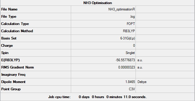
A molecule of NH3 was drawn on Gaussview and its 6-31G(d,p) optimisation was ran on Gaussian (*.log file can be found here) under the B3LYP method. C3v was forced using the opt=tight, scf=conver=9 and int=ultrafine keywords. A summary of such optimisation can be seen in Figure 11 and the logbook showing convergence follows.

       Item               Value     Threshold  Converged?
 Maximum Force            0.000005     0.000450     YES
 RMS     Force            0.000003     0.000300     YES
 Maximum Displacement     0.000010     0.001800     YES
 RMS     Displacement     0.000007     0.001200     YES
 Predicted change in Energy=-7.830518D-11
 Optimization completed.
    -- Stationary point found.
Frequency Analysis for NH3
The Frequency analysis was ran on Gaussian with the same parameters as the above optimisation. The complete *.log file can be found here, a summary can be seen in Figure 12 and the logbook entry showing convergence follows.

 Item               Value     Threshold  Converged?
 Maximum Force            0.000006     0.000015     YES
 RMS     Force            0.000004     0.000010     YES
 Maximum Displacement     0.000014     0.000060     YES
 RMS     Displacement     0.000009     0.000040     YES
 Predicted change in Energy=-1.141894D-10
 Optimization completed.
    -- Stationary point found.
The convergence to a minimum was checked by inspecting the sign of the low frequencies, that are indeed all positive. Additionally all the "near zero" frequencies are satisfactorily close to zero.
 Low frequencies ---   -0.0131   -0.0027   -0.0019    7.1039    8.1053    8.1056
 Low frequencies --- 1089.3834 1693.9368 1693.9368
Molecular Orbitals for NH3
An MO analysis calculation was set up from the optimised NH3 *.chk file. The method and basis set were the same but some parameters were changed: the full NBO option was selected under the relative tab and the keywords pop=full were added. This calculation was run on the HPC SCAN portal (DOI:10042/27748 ).
NBO analysis for NH3
We can analyse the NBOs from the *.log output of the above population analysis. The NBO charge distribution (with a specific color range between -1.132 to +1.132) can be seen in Figure 13, while the specific NBO charges for each atom are shown in Figure 14.

|

|
| Figure 13 | Figure 14 |
It is interesting to note that although we can represent the specific charges on each atom visually as above, these are also stored in the Gaussian output *.log file:
******************************Gaussian NBO Version 3.1******************************
             N A T U R A L   A T O M I C   O R B I T A L   A N D
          N A T U R A L   B O N D   O R B I T A L   A N A L Y S I S
 ******************************Gaussian NBO Version 3.1******************

Summary of Natural Population Analysis:

                                       Natural Population
                Natural  -----------------------------------------------
    Atom  No    Charge         Core      Valence    Rydberg      Total
 -----------------------------------------------------------------------
      N    1   -1.13220      1.99981     6.11805    0.01434     8.13220
      H    2    0.37740      0.00000     0.62045    0.00214     0.62260
      H    3    0.37740      0.00000     0.62045    0.00214     0.62260
      H    4    0.37740      0.00000     0.62045    0.00214     0.62260
 =======================================================================
   * Total *    0.00000      1.99981     7.97941    0.02078    10.00000
Since this is a neutral molecule, the sum of all specific charges is zero. The negative charge on N is due to the high electronegativity of N, which makes it withdraw electron density from the Hydrogen atoms, that in turn end up bearing a positive charge.
Association Energies: Ammonia Borane
The objective of this section was to compute the reaction energy for the following reaction:
When trying to compute a reaction energy, the basis set and method have to remain constant throughout reactant and products. The parameters used all throughout the following computations were:
- method: B3LYP
- basis set: 6-31G(d,p)
- additional keywords: opt=tight, scf=conver=9, int=ultrafine
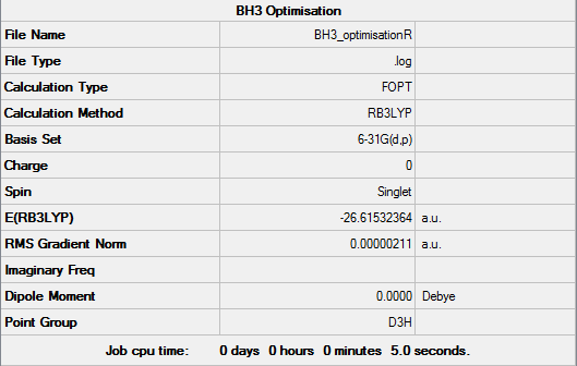
To ensure a continuity of computation level, NH3 and BH3 were re-optimised with the above settings. The *.log files can be found here and here respectively and the results are summarised here and here respectively.
Subsequently, a molecule of NH3BH3 was optimised on Gaussian at the same level (i.e. using the same parameters). The *.log file can be found here, a summary can be seen in Figure 15 and the logbook entry showing convergence follows.

Item               Value     Threshold  Converged?
 Maximum Force            0.000002     0.000015     YES
 RMS     Force            0.000001     0.000010     YES
 Maximum Displacement     0.000034     0.000060     YES
 RMS     Displacement     0.000010     0.000040     YES
 Predicted change in Energy=-1.180597D-10
 Optimization completed.
    -- Stationary point found.
A frequency analysis was also conducted on AmmoniaBorane, its *.log output file can be found here, a summary can be seen in Figure 16 and its logbook entry showing convergence follows.

Item               Value     Threshold  Converged?
 Maximum Force            0.000004     0.000450     YES
 RMS     Force            0.000001     0.000300     YES
 Maximum Displacement     0.000030     0.001800     YES
 RMS     Displacement     0.000014     0.001200     YES
 Predicted change in Energy=-1.357120D-10
 Optimization completed.
    -- Stationary point found.
The frequency analysis allowed to inspect the low frequencies and to deduce that the optimisation had indeed converged to a minimum. Additionally the "near zero" frequencies can be seen to be reasonably close to zero.
 Low frequencies ---   -3.2917   -1.8894   -0.0013   -0.0011   -0.0009    3.1013
 Low frequencies ---  263.4155  632.9554  638.4295
The energies of the optimised reactants and products can be found in the respective optimisation summaries and from these the bond dissociation energy can be calculated in a few straightforward steps.
Failed to parse (syntax error): {\displaystyle ΔE = E_{NH3BH3}-(E_{NH3}+E_{BH3}) = -83.22468908 – (-56.55778673 -26.61532364) = - 0.05157872 AU = - 0.05157872 * 2625.49962 kJ/mol = -135.4199098 kJ/mol }
The negative sign implies that the energy of NH3BH3 is lower than the sum of the energies of the reactants: this means that it is energetically favourable to form ammonia borane. Inversely +135.42 kJ/mol must be the dissociation energy of NH3BH3. We can take the fact that the bond energy is almost 55 times bigger than the thermal energy at room temperature (~2.5 kJ/mol), meaning that the bond is stable at room temperature, as an indication that the value we computed is sensible.
It is worth noting that the fact that this reaction is entropically disfavoured (as it involves the condensation of two moles of gas into one of solid) is not at all deducible from the calculations done up until now, which are only based on electronic and nuclear interactions.
Conclusion
Based on analysis of the computed structures and comparison with the literature, we can conclude that we have indeed successfully modeled BH3, GaBr3, NH3 and NH3BH3. Computational chemistry has allowed for the qualitative investigations into various properties of small complexes, in particular the vibrational modes of small molecules can be simulated quite fast and accurately.
Part 2: Ionic Liquids & Designer Solvents
Introduction
An ionic liquid is a salt in which the ions are poorly coordinated, which results in these solvents being liquid below 100°C, or even at room temperature (room temperature ionic liquids, RTIL's). Within the ionic liquid complex, one ion will have a delocalized charge and the other will be organic, preventing the formation of a stable crystal lattice. Their multi-component property allows them to be varied more easily depending on the properties needed in the solvent. Hence they are sometimes called "designer solvents".
This part of the module involved firstly the simulation of three small cations ([N(CH3)4]+, [P(CH3)4]+ and [S(CH3)3]+) to investigate the effect of varying central atoms on the geometries and NBO charges distributions. Successively bigger cations ([N(CH3)3(CH2OH)]+ and [N(CH3)3(CH2CN)]+ were optimised to be compared to the unsubstituted [N(CH3)4]+ to try and derive insights on the effect of EWGs and EDGs on the geometries, MOs and charge distributions. Additionally, an extra cation was optimised and investigated ([N(CH3)3(CH2CH2CN)]+), to investigate whether the distance between the substituent group and the central atoms matters or not and if so, how much.
Section A: Comparison of Selected "onium" Cations
Analysis of [N(CH3)4]+
Optimisation
Following the same considerations as when optimising neutral molecules, a positive [N(CH3)4]+ cation was optimised. The calculation was set up on Gaussview with the following parameters: B3LYP method, 6-31G(d,p) basis set, opt=tight, scf=conver=9, int=ultrafine keywords and the charge was set at +1. This set up was then sent to the HPC SCAN portal to be run (DOI:10042/27718 ), a summary is shown in Figure 17 and the logbook entry showing convergence follows.
4_optimisationdata.PNG)
     Item               Value     Threshold  Converged?
 Maximum Force            0.000095     0.000450     YES
 RMS     Force            0.000022     0.000300     YES
 Maximum Displacement     0.001470     0.001800     YES
 RMS     Displacement     0.000483     0.001200     YES
 Predicted change in Energy=-1.679456D-07
 Optimization completed.
    -- Stationary point found.
4_optimisedstructure.PNG)
The optimised structure can be seen in Figure 18 and the bond length and angles are summarized in Table 5.
The optimised molecule shows a tetrahedral geometry, and this is proven by the C-N-C bond angles, which are all between 109.457° and 109.484°, all close to value given by VSEPR analysis of ~109.48°.
The C-N bond lengths also range as expected between 1.50936 Å and 1.50950 Å (lit. value: 1.51 Å[6]), while all C-H bond lengths are comprised between 1.09015 Å and 1.09021 Å (coinciding with the literature values).
Frequency Analysis
A frequency analysis was then ran with the same parameters on the HPC SCAN portal (DOI:10042/27746 ). A summary is shown in Figure 19 and the logbook entry follows.
4_frequencydata.png)
Item               Value     Threshold  Converged?
 Maximum Force            0.000112     0.000450     YES
 RMS     Force            0.000038     0.000300     YES
 Maximum Displacement     0.002008     0.001800     NO
 RMS     Displacement     0.000659     0.001200     YES
 Predicted change in Energy=-1.773175D-07
As the frequency analysis did not actually fully converge, we have to decide if this is a problem or if the non-convergence is negligible. The first step is to check if the structure on which the frequency analysis has been conducted is actually the optimised structure. This is easily verified by checking the energy of the optimised molecule and the energy of the molecule on which the frequency analysis has been run: since they only differ by , a very insignificant amount, we can reasonably conclude that they have the same geometry.
Additionally, examining the logbook entry shows that the only Item that did not converge was the "Maximum displacement", and that the value at which Gaussian stopped was very close to the threshold.

These two observations lead to the deduction that [N(CH3)4]+ must have quite a flat Potential Energy Surface: the optimisation probably stopped before the minimum was actually reached, because the program was tricked by the very low curvature of the energy profile and by consequence by the gradient being very close to zero into thinking the optimisation was complete. Figure 20 shows the difference in gradient when trying to optimise a high curvature PES and a low curvature one.
An energy profile resembling the lowest energy PES shown in the diagram is what we think is the case for [N(CH3)4]+: the optimisation ends in a near-flat surface, and this "almost stationary" point differs from the "real minimum" only by a small displacement (hence the non-convergent displacement item found in the *.log file).
Since the low frequencies:
Low frequencies ---  -20.8664    0.0003    0.0004    0.0010   11.3410   17.7465
 Low frequencies ---  183.8383  287.2260  287.6116
do not show any imaginary vibrations we can assume this non-convergence is negligible and move on from here.
Analysis of [P(CH3)4]+
Optimisation
The [P(CH3)4]+ molecule was optimised using the same parameters as the above [N(CH3)4]+ cation, i.e. B3LYP method, 6-31G(d,p) and opt=tight, scf=conver=9 and int=ultrafine as additional keywords. Such calculation was submitted to th HPC SCAN portal (DOI:10042/27726 ), a summary can be seen in Figure 21 and the logbook entry showing convergence follows.
4_optimizationdata.PNG)
         Item               Value     Threshold  Converged?
 Maximum Force            0.000010     0.000015     YES
 RMS     Force            0.000003     0.000010     YES
 Maximum Displacement     0.000050     0.000060     YES
 RMS     Displacement     0.000015     0.000040     YES
 Predicted change in Energy=-4.116363D-10
 Optimization completed.
    -- Stationary point found.
4_optimisationstructure.PNG)
The optimised structure can be seen in Figure 22, it looks like the molecule has a tetrahedral geometry in its lowest energy conformation. Confirmation of this hypothesis is given by inspection of the C-P-C bond angles, which are indeed all between 109.467° and 109.472°, as expected from VSEPR theory.
All bond lenghts are also relatively consistent with respect to each other and with respect to literature values: all C-P bonds range between 1.81637 Å and 1.81640 Å (lit. value: 1.81 Å[7]), while all C-H bonds have lengths comprised between 1.09329 Å and 1.09330 Å.
A population analysis was then run on the HPC SCAN portal with the same setting as the other similar calculations run within this experiment (DOI:10042/27755 ).
Frequency Analysis
The optimisation of [P(CH3)4]+ was used as a starting point for a Frequency Analysis ran using the same parameters. After being set up through GaussView, this computation was sent to the HPC SCAN portal (DOI:10042/27747 ). A summary of the analysis can be seen in Figure 23 and the logbook entry showing convergence follows.
4_frequencydata.PNG)
Item               Value     Threshold  Converged?
 Maximum Force            0.000012     0.000450     YES
 RMS     Force            0.000004     0.000300     YES
 Maximum Displacement     0.000631     0.001800     YES
 RMS     Displacement     0.000211     0.001200     YES
 Predicted change in Energy=-4.131587D-09
 Optimization completed.
    -- Stationary point found.
A closer look to the *.log file confirmed the convergence to a minimum: the so-called "near zero" frequencies were indeed reasonably close to zero and no negative vibrational mode was reported.
Low frequencies ---   -0.0021    0.0010    0.0016    7.2514    7.6867   10.3173
Low frequencies ---  156.3963  191.5237  191.5604
Analysis of [S(CH3)3]+
Optimisation
The third cation examined was [S(CH3)3]+. This molecule was also optimised by setting up a B3LYP calculation (6-31G(d,p) method, opt=tight, scf=conver=9 and int=ultrafine keywords) on GaussView. This calculation was also sent to the HPC SCAN portal (DOI:10042/27730 ), a summary can be seen in Figure 24 amd the logbook entry showing convergence follows.
3_optimisationdata.PNG)
         Item               Value     Threshold  Converged?
 Maximum Force            0.000007     0.000015     YES
 RMS     Force            0.000002     0.000010     YES
 Maximum Displacement     0.000055     0.000060     YES
 RMS     Displacement     0.000015     0.000040     YES
 Predicted change in Energy=-2.974872D-10
 Optimization completed.
    -- Stationary point found.
3_optimisationstructure.PNG)
The optimised structure can be seen in Figure 25. This molecule is also tetrahedral but differs from the two previously observed cations because one of the four electron pairs is not involved in bonding but rather resides in the valence shell. The observed bond angle value is between 102.741° and 102.747°and can be rationalised by remembering that from valence theory a lone pair exerts more repulsion than a bond pair.This means that the LP pushes the methyl groups away more strongly and thus reduces the amplitude of the angles within them. These angles are therefore smaller than the ideal tetrahedral bond angles.
The bond lengths are reasonably consistent, with the S-C bonds ranging from 1.82262 Å to 1.82264 Å (lit. value: 1.82 Å [8]) and the C-H bonds falling within a range between 1.09158 Å and 1.09159 Å.
A population analysis was then run on the HPC SCAN portal with the usual parameters and keywords. The complete output file was published under the following DOI:10042/27760
Frequency Analysis
A Frequency Analysis was run from the above optimised [S(CH3)3]+ structure, keeping the same parameters. Such Frequency computation was sent to the HPC SCAN portal (DOI:10042/27753 ), a summary can be seen in Figure 26 and the logbook entry showing convergence follows.
3_frequencydata.PNG)
Item               Value     Threshold  Converged?
 Maximum Force            0.000005     0.000450     YES
 RMS     Force            0.000002     0.000300     YES
 Maximum Displacement     0.001152     0.001800     YES
 RMS     Displacement     0.000345     0.001200     YES
 Predicted change in Energy=-4.385233D-09
 Optimization completed.
    -- Stationary point found.
A closer inspection of the *.log file gives an opportunity to check that the optimisation converged to a minimum. We can see that, as we would expect in this case, the "near zero" frequencies are reasonably low and all vibrational modes are positive and hence real.
Low frequencies ---  -10.0083   -1.4923   -0.0039   -0.0037    0.0032   16.3350
 Low frequencies ---  162.2088  199.4735  199.6829
MO analysis for [N(CH3)4]+
A population analysis was set up and ran on the HPC SCAN portal with the dame settings as all the other population analyses conducted within this module (DOI:10042/27752 ). Its output file permitted the visualisation of some interesting MOs through GaussView's graphical interface. The discussion of the Atomic Orbital interactions in 5 of these MOs is presented in Table 5.
| MO #6 | MO #10 | MO #13 |
4_MO6_interactions.PNG) |
4_MO10_interactions.PNG) |
4_MO13_interactions.PNG) |
| MO #16 | MO #19 | |
4_MO16_interactions.PNG) |
4_MO19_interactions.PNG) |
As can be seen in the above table, MO #6 is very delocalised, contains no nodes and is very bonding overall, due to very strong AO interactions and weaker through-space ones. In contrast, MO #10 presents four angular nodal planes and in addition to the strong AO bonding interactions within the orbital lobes (which are not shown in the picture) also contains strong through-space interaction, both bonding (between orbital lobes in the same phase) and antibonding (between lobes in opposite phases. MO #13 has three angular nodal planes and less bonding interactions (except for the AO interactions due to core atom-atom interactions), but strong through-space antibonding interactions are clearly visible. We can see four angular nodal planes in MO #16, and a lot of strong through-space interactions (both bonding and antibonding). MO #19 shows angular nodal planes at every C-N junction and, in addition to very strongly bonding through-space interactions, some weakly bonding through-space interactions are also visible.
Comparison and Analysis of the Contributions of each Atom to Bonding across the Three Cations
| NBO charge distribution | NBO specific charges (graphical description) |
|---|---|
4_NBOdata.PNG) |
4_chargedata.PNG)
|
| NBO charge distribution | NBO specific charges (graphical description) |
|---|---|
4_NBOdata.PNG) |
4_chargedata.PNG)
|
| NBO charge distribution | NBO specific charges (graphical description) |
|---|---|
3_NBOdata.PNG) |
3_chargedata.PNG)
|
GaussView can read the output of the population analysis to give a graphical description of the charge distribution over each cation, as seen in Table 6 . Additionally, the output file can be opened to show a detailed charge distribution, also shown in Table 6. By observing the specific charges carried by the atoms in each cation, we can see that while N is negatively charged, P and S carry a positive charge. However, since all central atoms donate an electron pair to be able to bond with the Carbon atoms, they are all electron deficient. This can be rationalised by considering the similar size of N and C, similarity that gives a better orbital overlap. This factor, added to the higher elecronegativity of N when compared to P or S contributes to the Nitrogen's inductive effect, which allows it to be negatively charged.
On the contrary, S and P do not show signs of inductive effect, since they have more mismatched and larger orbitals, that do no overlap very well with the orbitals on the Carbon atoms. They also have electronegativity values that are the same (Sulfur) or lower (Phosphorus) than that of Carbon, which means that they will undergo electron pair donation and therefore be positively charged.
The negative charge values of the Carbon atoms (due to the electron-withdrawing effect on the Hydrogens' densities) arises from the need to balance the positive charge present on the heteroaroms and is in fact directly proportional to it. Hence the C in [N(CH3)4]+ will have the lowest charge value, followed by the C in [P(CH3)4]+ and then finally those in [S(CH3)3]+.
| [N(CH3)4]+ |
1. (1.99118) BD ( 1) All C-H bonds: ( 63.47%) 0.7967* C s( 26.42%)p 2.78( 73.53%)d 0.00( 0.05%) ( 36.53%) 0.6044* H s( 99.95%)p 0.00( 0.05%) 4. (1.98452) BD ( 1) All C-N bonds: ( 33.65%) 0.5801* C s( 20.77%)p 3.81( 79.07%)d 0.01( 0.16%) ( 66.35%) 0.8146* N s( 25.00%)p 3.00( 74.97%)d 0.00( 0.03%) |
| [S(CH3)3]+ |
1. (1.98721) BD ( 1) All C-H bonds: ( 64.83%) 0.8051* C s( 26.50%)p 2.77( 73.45%)d 0.00( 0.05%) ( 35.17%) 0.5931* H s( 99.95%)p 0.00( 0.05%) 4. (1.98631) BD ( 1) All C-S bonds: ( 48.67%) 0.6976* C s( 19.71%)p 4.07( 80.16%)d 0.01( 0.14%) ( 51.33%) 0.7165* S s( 16.95%)p 4.86( 82.42%)d 0.04( 0.63%) |
| [P(CH3)4]+ |
1. (1.98385) BD ( 1) All C-H bonds: ( 64.78%) 0.8049* C s( 24.88%)p 3.02( 75.08%)d 0.00( 0.04%) ( 35.22%) 0.5934* H s( 99.95%)p 0.00( 0.05%) 4. (1.98030) BD ( 1) All C-P bonds: ( 59.57%) 0.7718* C s( 25.24%)p 2.96( 74.67%)d 0.00( 0.08%) ( 40.43%) 0.6358* P s( 25.00%)p 2.97( 74.15%)d 0.03( 0.85%) |
The first set of informative data deducible from Table 7 is the hybridisation of all the atoms present in the molecules under investigation. Since the C-H bonds are effectively all the same, we will focus on the different C-X bonds. We can see that N and P are clearly sp3 hybridised, while S and C (in all bonds) are in a similar, but not as well defined, hybridisation state. Table 7 also allows us to analyse the relative orbital contribution of the C and heteroatom to the C-X bond. Since all three molecules are symmetrical the following discussion on one C-X bond can be applied to all three (or four) such bonds present in the molecules.
We can see that we cover all the possible "patterns of bond sharing": P contributes less (about 40 %) than C to the C-P bond, S and C share their bond almost 50:50 and N contributes more (ca. 80%) than C to the C-N bond. This effect mirrors the electronegativity trends discussed in the previous paragraphs: N has the highest electronegativity so it is the heteroatom that is most capable out of the three to hold on tightly to its electron density, and as such it contributes the most to the bond with C. This also means that the dipole moment points towards N and as a result the C-N bond is expected to be polar.
Additionally C and S are close in the electronegativity scale, hence they share their bond quite fairly. We can therefore expect the C-S bond to be less polar than the other two.
P is electropositive with respect to the Carbon atoms and only able to contribute by less than half to the bond character,so the C-P bond is polarised towards the C atom. This is an indication that the electron density is higher around the C atom and so the positive charge on P described above can be further rationalised as a region of lower electron density.
Discussion on the formal charge of [N(CH3)4]+
Tetra-alkyl cations are usually represented with a positive charge on the nitrogen centre. However the calculations done on [N(CH3)4]+ discussed above dismiss this description. Although the "formal" positive charge on the N represents its electron donation to the fourth methyl group, we know from the charge distribution analysed within the population discussion that in fact it is the hydrogens that are positively charged, and as such should bear the positive charge when drawn out. It is worth pointing out that such a drawing would be quite impractical (as each of the 12 H atoms would need to show some positive character) and an ideal compromise is probably that of drawing the Nitrogen cation between square brackets and drawing the positive charge outside them.
Section B: Influence of Functional Groups
Analysis of [N(CH3)(CH2OH)]+
Optimisation
A bigger cation was then submitted for analysis. As usual, the first calcultation to be run was an optimisation. The following parameters were used:
- B3LYP method
- 6-31G(d,p) basis set
- opt=tight, scf=conver=9, int=ultrafine additional keywords.
This optimisation was sent to the HPC SCAN portal (DOI:10042/27784 ), a summary can be seen in Figure 27 and the logbook entry showing convergence follows.
3(CH2OH)_optimisationdata_wrong.PNG)
Item               Value     Threshold  Converged?
 Maximum Force            0.000001     0.000015     YES
 RMS     Force            0.000001     0.000010     YES
 Maximum Displacement     0.000030     0.000060     YES
 RMS     Displacement     0.000008     0.000040     YES
 Predicted change in Energy=-8.012853D-11
 Optimization completed.
    -- Stationary point found.
3(CH2OH)_optimisationstructure_wrong.PNG)
The optimised structure can be seen in Figure 28 The optimised structure is shown in Figure 28, in which the Nitrogen atom and the Hydrogen atom on the Hydroxy group have a dihedral angle of 180°. Some bond lengths have been inspected via GaussView and are reported here and are all consistent with literature values:
- O-H : 1.38667 Å
- C13-N : 1.52089 Å
- C5-N and C6-N : 1.51228 Å
- C1-N : 1.50620 Å
- C-H bonds range between 1.08769 Å and 1.09758 Å.
It might be worth noting that although all bond length value are relatively close, the longest C-N bond is the one to the only Carbon atom bound to the Oxygen, and that the shortest of such bonds is the one directly opposite to it. Additionally, the longest C-H bonds (with exactly the same value) are also the ones to the Carbon bearing the hydroxy group.
The values of the optimised bond angles are as expected: the O-C-N bond is around 106.1°, while the C-N-C are only slightly larger than what predicted by VSEPR, ranging between 109.624° to 109.778° (incidentally, the smallest angles are the ones that include C13).
Frequency Analysis
Running a frequency analysis from the previously optimised molecule incurred in a problem, as (albeit being reasonably convergent) the "near zero" frequencies resulted too large to be acceptable (outside the ±30 cm-1 range that allows for the specific very soft vibrational modes) and picked up an "imaginary" negative vibration frequency:
Item               Value     Threshold  Converged?
 Maximum Force            0.000048     0.000450     YES
 RMS     Force            0.000017     0.000300     YES
 Maximum Displacement     0.001888     0.001800     NO
 RMS     Displacement     0.000600     0.001200     YES
 Predicted change in Energy=-5.001837D-08

 Low frequencies --- -124.9600  -16.0197   -6.4784    0.0003    0.0008    0.0008
 Low frequencies ---    7.6597  125.8047  212.3054
 ******    1 imaginary frequencies (negative Signs) ******
When examining the vibrational movements to pinpoint which atoms were being problematic, it could be observed that the frequency coming up as negative was the one down to the movement of the Hydrogen atom bound to the Oxygen.
To correct for this issue, the optimised *.log file was reopened and the dihedral angle between the terminal Hydrogen and the Nitrogen was changed from 180° to about 150°, and the molecule was successively set up to be reoptimised with the same parameters as the first optimisation.
The calculation was then sent to the HPC SCAN portal (DOI:10042/27785 ). A summary of such calculation is shown in Figure 29 and the logbook entry showing convergence follows.
3(CH2OH)_optimisationdata.PNG)
Item               Value     Threshold  Converged?
 Maximum Force            0.000001     0.000015     YES
 RMS     Force            0.000000     0.000010     YES
 Maximum Displacement     0.000038     0.000060     YES
 RMS     Displacement     0.000010     0.000040     YES
 Predicted change in Energy=-2.469228D-11
 Optimization completed.
    -- Stationary point found.
3(CH2OH)_optimisedstructure.PNG)
The newly optimised structure is shown in Figure 30.
A second frequency analysis was set up from this new optimisation,still keeping the same parameters. This time around the results were acceptable (low "near zero" frequencies and positive vibration frequencies showing that the optimisation actually converged to a minimum). What these results show is that the first optimisation probably converged to a transition state: still a stationary point, but this time a maximum, explaining why the second derivative (the frequency analysis) yielded a negative value. This is why changing the O-C-N angle ever so slightly makes the optmisation fall down to a minimum. This computation was run on the HPC SCAN portal (DOI:10042/27787 ), a summary can be seen in Figure 31 and the logbook entry showing convergence follows. The "low frequencies" section of the *.log file is also shown.
3(CH2OH)_frequencydata.PNG)
Item               Value     Threshold  Converged?
 Maximum Force            0.000002     0.000450     YES
 RMS     Force            0.000001     0.000300     YES
 Maximum Displacement     0.000076     0.001800     YES
 RMS     Displacement     0.000026     0.001200     YES
 Predicted change in Energy=-6.221953D-12
 Optimization completed.
    -- Stationary point found.
Low frequencies ---   -8.4482   -5.0138   -1.1682   -0.0007   -0.0004   -0.0004
 Low frequencies ---  131.1088  213.4679  255.7114
NBO Analysis
3(CH2OH)_chargedistribution.PNG)
3(CH2OH)_NBOcharges.PNG)
A population analysis was then run, using the formatted checkpoint file of the second optimisation of the cation. Such energy computation was set up with the similar parameters to the optimisation and frequency analysis: B3LYP method and 6-31G(d,p) basis set, but with the full NBO set up and the additional keyword pop=full was added. This calculation was run on the HPC SCAN portal (DOI:10042/27790 ), and its *.log file was opened in GaussView to visualize the NBO charges. There are two ways of visualising such charges in GaussView: as charge distribution or by giving each atom a specific charge and then showing such on the structure itself. Additionally the *.log file can also be opened separately and the specific charge information can be found and listed. The charge distribution is shown in Figure 32 (note that the color range is between -1 and 1), and the specific charges are both shown visually in Figure 33 and copied from the *.log file.
Summary of Natural Population Analysis:

                                       Natural Population
                Natural  -----------------------------------------------
    Atom  No    Charge         Core      Valence    Rydberg      Total
 -----------------------------------------------------------------------
      C    1   -0.49215      1.99946     4.47855    0.01414     6.49215
      H    2    0.26882      0.00000     0.73010    0.00108     0.73118
      H    3    0.26640      0.00000     0.73251    0.00109     0.73360
      H    4    0.27385      0.00000     0.72511    0.00105     0.72615
      C    5   -0.49384      1.99946     4.47920    0.01518     6.49384
      C    6   -0.49141      1.99946     4.47693    0.01501     6.49141
      H    7    0.27099      0.00000     0.72710    0.00190     0.72901
      H    8    0.27212      0.00000     0.72688    0.00099     0.72788
      H    9    0.26204      0.00000     0.73692    0.00104     0.73796
      H   10    0.26645      0.00000     0.73254    0.00100     0.73355
      H   11    0.28246      0.00000     0.71597    0.00156     0.71754
      H   12    0.26565      0.00000     0.73334    0.00101     0.73435
      C   13    0.08846      1.99939     3.88520    0.02695     5.91154
      H   14    0.23743      0.00000     0.76102    0.00156     0.76257
      H   15    0.24902      0.00000     0.74922    0.00177     0.75098
      O   16   -0.72546      1.99981     6.71322    0.01243     8.72546
      H   17    0.52074      0.00000     0.47551    0.00375     0.47926
      N   18   -0.32160      1.99949     5.31497    0.00714     7.32160
 =======================================================================
   * Total *    1.00000     11.99708    37.89428    0.10864    50.00000
Analysis of [N(CH3)(CH2CN)]+
Optimisation
The cation was firstly drawn on GaussView and then set up to be optimised. The parameters used were the usual ones: B3LYP method, 6-31G(d,p) basis set and opt=tight, scf=conver=9 and int=ultrafine as additional keywords. The calculation was run on the HPC SCAN portal (DOI:10042/27762 ), a summary is shown in Figure 34 and the logbook entry showing convergence follows.
3(CH2CN)_optimisationdata.PNG)
Item               Value     Threshold  Converged?
 Maximum Force            0.000000     0.000015     YES
 RMS     Force            0.000000     0.000010     YES
 Maximum Displacement     0.000004     0.000060     YES
 RMS     Displacement     0.000001     0.000040     YES
 Predicted change in Energy=-8.496971D-13
 Optimization completed.
    -- Stationary point found.
3(CH2CN)_optimisationstructure.PNG)
The optimised structure can be seen in Figure 35. Inspection of bond angles gives some interesting insights. While the N17-C-C bond angle is not surprisingly ~180°, we might expect all C-N18-C angles to fit a tetrahedral geometry (i.e. to all have a value similar to ~109.5°. In reality inspection via GaussView reveals that even tho the angles that do not involve the substituted Carbon atom (C13) do have a similar angle between them, the three angles that do involve C13 are larger than expected (albeit only by about 1.5°).
Inspection of the various bond lengths within this cations yields values that all align with the literature, except for the surprisingly short C13-C16 bond length (1.46 vs. 1.54 Å, probably due to the polarising effect of the nitrile unit).
Frequency Analysis
The above optimisation was then used to run a Frequency Analysis, set up with the same parameters. This computation was also sent to the HPC SCAN portal (DOI:10042/27765 ), a summary can be seen in Figure 36 and the logbook entry showing convergence follows.
3(CH2CN)_frequencydata.PNG)
Item               Value     Threshold  Converged?
 Maximum Force            0.000001     0.000450     YES
 RMS     Force            0.000000     0.000300     YES
 Maximum Displacement     0.000078     0.001800     YES
 RMS     Displacement     0.000018     0.001200     YES
 Predicted change in Energy=-4.434054D-11
 Optimization completed.
    -- Stationary point found.
Additionally, analysis of the *.log file allowed to confirm that the optimisation converged to a minimum: the "near zero" frequencies are all within a reasonable range and the vibration frequencies are all real and positive.
Low frequencies ---   -2.6164   -0.0008   -0.0006    0.0003    7.1487    9.6726
 Low frequencies ---   91.7740  154.0267  210.9300
NBO Analysis
The optimisation *.fchk file was used to set up a population analysis. Such energy calculation was set up using the same method and basis set as the optimisation, but replacing the additional keywords with pop=full and making sure the full-NBO option was selected. After being set up on GaussView, this computation was run on the HPC SCAN portal (DOI:10042/27766 ).
The resulting output file was then used to inspect the NBO charges on the cation. Such charges are shown as a charge distribution in Figure 37 (within a color range of -1 to +1) and are also listed as specific charges.
3(CH2CN)_chargedistribution.PNG)
Summary of Natural Population Analysis:

                                       Natural Population
                Natural  -----------------------------------------------
    Atom  No    Charge         Core      Valence    Rydberg      Total
 -----------------------------------------------------------------------
      C    1   -0.48854      1.99946     4.47441    0.01468     6.48854
      H    2    0.26948      0.00000     0.72951    0.00101     0.73052
      H    3    0.28206      0.00000     0.71681    0.00113     0.71794
      H    4    0.27375      0.00000     0.72527    0.00098     0.72625
      C    5   -0.48854      1.99946     4.47441    0.01468     6.48854
      C    6   -0.48530      1.99946     4.47115    0.01468     6.48530
      H    7    0.26948      0.00000     0.72951    0.00101     0.73052
      H    8    0.27375      0.00000     0.72527    0.00098     0.72625
      H    9    0.28206      0.00000     0.71681    0.00113     0.71794
      H   10    0.27686      0.00000     0.72218    0.00096     0.72314
      H   11    0.27074      0.00000     0.72824    0.00101     0.72926
      H   12    0.27074      0.00000     0.72824    0.00101     0.72926
      C   13   -0.35763      1.99915     4.34259    0.01589     6.35763
      H   14    0.30884      0.00000     0.68973    0.00143     0.69116
      H   15    0.30884      0.00000     0.68973    0.00143     0.69116
      C   16    0.20868      1.99940     3.75873    0.03319     5.79132
      N   17   -0.18624      1.99966     5.16584    0.02074     7.18624
      N   18   -0.28904      1.99950     5.28314    0.00641     7.28904
 =======================================================================
   * Total *    1.00000     13.99608    39.87159    0.13233    54.00000
Analysis of [N(CH3)(CH2CH2CN)]+
Optimisation
The larger cation was drawn on GaussView and set up to be optimised with the usual parameters: B3LYP method, 6-31G(d,p) basis set and opt=tight, scf=conver=9 and int=ultrafine. Such optimisation was then sent to be run on the HPC SCAN portal (DOI:10042/27782 ). A summary is shown in Figure 38 and the logbook entry showing convergence follows.
(CH2CH2CN)_optimisationdata.PNG)
         Item               Value     Threshold  Converged?
 Maximum Force            0.000000     0.000015     YES
 RMS     Force            0.000000     0.000010     YES
 Maximum Displacement     0.000013     0.000060     YES
 RMS     Displacement     0.000004     0.000040     YES
 Predicted change in Energy=-5.287643D-12
 Optimization completed.
    -- Stationary point found.
(CH2CH2CN)_optimisedstructure.PNG)
The structure of the optimised molecule is shown in Figure 39. Analysis of the optimised bond angles shows an almost perfectly tetrahedral central Nitrogen atom (albeit some deviation from ideality are present in the bond angles that involve C13, which are a little bit larger than 109.5°). It also shows a practically linear (~177°) C-C-N21 bond and indicates that the N18-C13-C14 and C13-C14-C28 angles are both simil-tetrahedral in character (about 3° larger than an ideal tetrahedral angle). Last but not least, we can try to approximate the angle between the two Nitrogen atoms by imagining a N-C14-N bond angle and inspection shows this angle to be ~97°, which can be rationalised by thinking that the molecule with the lowest energy will be the one in which the two Nitrogen groups are as far as possible, but with the highest simmetry (and an orthogonal positioning would fit these criteria).
The only "anomalous" result coming from inspecting the various bond lenghts is the shorter than normal C14-C28 bond (1.47 vs 1.54 Å). This is due to the strong polarising effect of the nitrile unit.
Frequency Analysis
The optimised structure of the cation was used to compute a Frequency analysis. The same parameters were used, and the calculation was sent to the HPC SCAN centre to be run (DOI:10042/27783 ). A summary is shown in Figure 40 and the logbook entry showing near convergence follows.
(CH2CH2CN)_frequencydata.PNG)
         Item               Value     Threshold  Converged?
 Maximum Force            0.000002     0.000450     YES
 RMS     Force            0.000001     0.000300     YES
 Maximum Displacement     0.002013     0.001800     NO
 RMS     Displacement     0.000425     0.001200     YES
 Predicted change in Energy=-2.013039D-09
 Optimization completed on the basis of negligible forces.
    -- Stationary point found.
It is noticeable that the optimisation conducted during the frequency analysis hasn't fully converged, but since the difference between value and threshold is only about 12% of the latter, we (and Gaussian) can conclude the divergence is negligible.
A further proof of the quality optimisation is the analysis of the low frequencies, of which the "near zero" ones are very small for a molecule of this size. In addition, the vibration frequencies are all positive, showing that the optimisation actually converged to a minimum.
Low frequencies ---   -3.9435   -0.0011   -0.0011   -0.0006    4.5385    7.6358
 Low frequencies ---   40.2875  133.6993  191.1961
NBO Analysis
The formatted checkpoint file for the optimised cation was then used to run a population analysis. Such energy calculation was set up with the same method and basis set as the optimisation, but had only pop=full as an additional keyword. Additionally, the NBO option full=NBO was selected. This calculation was run on the HPC SCAN portal (DOI:10042/27799 ) and yielded a *.log file readable by GaussiView.
This *.log file allowed GaussView to display graphically the NBO charge distribution within the cation (ranging from -1 to +1, shown in Figure 41) and also gave specific information with regards to the charge carried by each atom, information that has been listed here.
(CH2CH2CN)_chargedistribution.PNG)
Summary of Natural Population Analysis:

                                       Natural Population
                Natural  -----------------------------------------------
    Atom  No    Charge         Core      Valence    Rydberg      Total
 -----------------------------------------------------------------------
      C    1   -0.48575      1.99944     4.47170    0.01461     6.48575
      H    2    0.26611      0.00000     0.73289    0.00100     0.73389
      H    3    0.28137      0.00000     0.71639    0.00224     0.71863
      H    4    0.26751      0.00000     0.73144    0.00105     0.73249
      C    5   -0.49057      1.99946     4.47652    0.01459     6.49057
      C    6   -0.48357      1.99947     4.46992    0.01419     6.48357
      H    7    0.26524      0.00000     0.73372    0.00104     0.73476
      H    8    0.27422      0.00000     0.72475    0.00103     0.72578
      H    9    0.27270      0.00000     0.72615    0.00115     0.72730
      H   10    0.27213      0.00000     0.72686    0.00101     0.72787
      H   11    0.26702      0.00000     0.73198    0.00100     0.73298
      H   12    0.27016      0.00000     0.72884    0.00101     0.72984
      C   13   -0.25554      1.99931     4.23959    0.01664     6.25554
      C   14   -0.59720      1.99914     4.58808    0.00998     6.59720
      H   15    0.27714      0.00000     0.72125    0.00161     0.72286
      H   16    0.27875      0.00000     0.71964    0.00162     0.72125
      H   17    0.32792      0.00000     0.67061    0.00147     0.67208
      H   18    0.29959      0.00000     0.69890    0.00151     0.70041
      N   19   -0.29831      1.99949     5.29229    0.00653     7.29831
      C   20    0.24371      1.99939     3.72303    0.03388     5.75629
      N   21   -0.25262      1.99964     5.23208    0.02090     7.25262
 =======================================================================
   * Total *    1.00000     15.99535    45.85661    0.14804    62.00000
Discussion on the Effect of different Functional Groups and distance from Central Atom on Charge Distribution
The Cyano group is an electron withdrawing group (EWG, or electron acceptor), while the Hydroxy group is an electron donating group (EDG, or electron donor). The former decreases the electron density in the Carbon atom it is directly bound to, making it electrophilic. On the contrary the latter increases the total electron density in the system, making the carbon atom to which the group is attached to more nuclephilic. This second type of substituent groups can help stabilise cations, while EWG help to stabilise anions.
The main observation that can be made when looking at charge distribution in thee three cations is the variation of the charge held by the Carbon atom bearing the heteroatom. This Carbon is neutrally charged in the Hydroxy-group containing cation, and positively charged in the two Cyano-containing cations. This can be rationalised by considering the different pull on electron density for each substituent, discussed above.
Rationalising the effect of distance on the charge distribution requires inspection of the *.log files to see if there is any change in the specific charges on each atom.
The specific charge value that will reflect the changes in differences most effectively is the charge on C(13), i.e. the Carbon in the substituted group that is directly bound to the central Nitrogen. We can see how there is less electron density on this Carbon in the biggest cation, but a higher negative charge on the Carbon directly bound to it, i.e. the Carbon that effectively lengthens the cation. A possible reason for this is that while C(13) in the "shorter" cation is sandwiched between the central atom and the cyano group, the longer hydrocarbon chain "traps" the electron density that therefore hovers around the C atoms without being pulled anywhere else.
MO Comparison between [N(CH3)(CH2OH)]+, [N(CH3)4]+, [N(CH3)(CH2CN)]+ and [N(CH3)(CH2CH2CN)]+
| [N(CH3)(CH2OH)]+ | [N(CH3)4]+ | |
| HOMO | 3(CH2OH)_HOMO.PNG) |
4_HOMO.PNG) |
| EHOMO | -0.48763 (-1280.27 kJ/mol) | -0.57930 (-1520.95 kJ/mol) |
| LUMO | 3(CH2OH)_LUMO.PNG) |
4_LUMO.PNG) |
| ELUMO | -0.12459 AU (-327.11 kJ/mol) | -0.13303 (-349.27 kJ/mol) |
| ΔE | 0.36304 (953.16 kJ/mol) | 0.44627 (1171 kJ/mol) |
| [N(CH3)(CH2CN)]+ | [N(CH3)(CH2CH2CN)]+ | |
| HOMO | 3(CH2CN)_HOMO.PNG) |
(CH2CH2CN)_HOMO.PNG) |
| EHOMO | -0.50048 (-1314.01 kJ/mol) | -0.47326 (-1242.54 kJ/mol) |
| LUMO | 3(CH2CN)_LUMO.PNG) |
(CH2CH2CN)_LUMO.PNG) |
| ELUMO | -0.18183 (-477.39 kJ/mol) | -0.14074 (-369.51 kJ/mol) |
| ΔE | 0.31865 (836.61 kJ/mol) | 0.33252 (873.03 kJ/mol) |
Table YYY summarises the shape and energies of the HOMO and LUMO orbitals of four of the cations that were under analysis in this module.
The first axis of comparison under consideration is the variation in shape of the various HOMO orbitals when one of the substituent varies from CH3 to CH2OH to CH2CN to CH2CH2CN. As before there are two variants in this system of cations: the electron withdrawing or donating effects of the substituent groups and the distance of such substituent group, investigated only for the cyano-containing cation.
Observing the shape of the HOMO orbitals helps us rationalise the energy ordering of the four cations, that indicates a [N(CH3)4]+ > [N(CH3)3(CH2CN)]+ > [N(CH3)3(CH2OH)]+ > [N(CH3)3(CH2CH2CN)]+ order of stability.
We can notice that the non-substituted cation contains weak bonding AO interactions, thrugh-space strong antibonding interactions(between orbital lobes in opposite phases) and weak bonding ones (where neighboring or near orbital lobes are in the same phase). Additionally the MO presents some delocalised character and each atom is the center of an angular nodal plane.
The shorter Cyano-substituted cation is almost entirely non-bonding, expect for the through-space antibonding π interactions around the linear part of the molecule. However this molecular orbital is overall weakly bonding, maybe due to the strong bonding interactions within the nitrile unit (the same interactions that yield the triple bond between the C and the N atom. This orbital is very localised.
The Hydroxy-substituted cation presents mainly antibonding through space interactions across the whole molecule, although some bonding ones can be seen between the orbital lobes on the methyl groups. Delocalisation is only present minorly over the CH2-OH unit.
The longer Cyano-substituted cation is very similar to its shorter counterpart, but slightly less antibonding which is probably a reason for its higher energy.
These results lead us to conclude that adding an electron donating OH group destabilised the HOMO of [N(CH3)4]+ by about 240 kJ/mol, while the addition of a cyano- electron withdrawing group destabilised the HOMO of the non-substituted cation by ~205 kJ/mol or ~280 kJ/mol for the longer cation.
The shape and energies of the four LUMOs can also be compared and the same kind of analysis done on the HOMOs can be applied. The order of stability is [N(CH3)3(CH2CN)]+ > [N(CH3)3(CH2CH2CN)]+ > [N(CH3)4]+ >[N(CH3)3(CH2OH)]+ this time around. This order presents several differences with the trend seen in the HOMOs, these differences can be rationalised by examining the shape of the MOs in question.
The exceptional stability of the LUMO of [N(CH3)3(CH2CN)]+ can be explained by the very favourable in-phase overlap across the CN-CH2 fragment and also across the orbital lobes on the methyls that are in the same phase. The reason why this orbital stays antibonding is the presence of very strong through-space antibonding interactions.
The LUMO of the longer CN-containing cation is also stabilised by the strong AO interactions around the central atom. When compared to its shorter counterpart these interactions actually seem stronger, due to the possibility to overlap with the orbital lobe in the same phase on the extra -CH2- group. This factor, which might lead to predicting a higher stability, is contrasted by the higher number of very strong through-space antibonding interactions, which also explain why this MO is antibonding overall.
In [N(CH3)4]+ the LUMO seems to present a very strong central region of AO bonding interactions but closer analysis leads to noticing that these are only due to the favorable overlap of the lobes on the Hydrogen atoms and as such must be quite weak. In contrast, the through-spaces antibonding interactions present across the 4 nodal planes at the C-N junctions are very strong and give the orbital its instable character.
The OH-containing cation mostly presents through-space antibonding interactions,pretty much the same as in the non-substituted cation, with the addition of a very strong region of through-space antibonding interactions around the H-O-CH2-N unit.
To put things in a quantitative perspective, adding a CN group close to the central atom of a [N(CH3)4]+ cation stabilises it by ~130 kJ/mol, while adding the same substituent but farther from the central atom has a weaker effect and stabilises it by only ~30 kJ/mol. On the contrary, adding an electron donating group destabilises the previously non-substituted cation by ~20 kJ/mol.
The last comparison we can make revolves around the change in the size of the HOMO-LUMO gap on substituent addition and variation. The energy gap in the [N(CH3)4]+ cation is around 1170 kJ/mol, and it gets reduced by about 220 kJ/mol when the OH- unit is substituted and by respectively ~340 kJ/mol and ~300 kJ/mol when the "short" and "long" versions of the CN substituting units are introduced. Since a smaller gap means an increased of conjugation in the system it can be concluded that both EDG and EWG substitution increase the conjugation level or a certain molecule, that CN- substituents do more so than OH- ones and that an increase in length only slightly dampens such effect.
References
- ↑ 1.0 1.1 1.2 http://scitation.aip.org/content/aip/journal/jcp/96/5/10.1063/1.461942
- ↑ PAC, 1994, 66, 1077 (Glossary of terms used in physical organic chemistry (IUPAC Recommendations 1994)) on page 1089
- ↑ 3.0 3.1 D.R. Lide, CRC Handbook of Chemistry and Physics, CRC Press, Boca Raton, 87th Ed., 2006
- ↑ 4.0 4.1 K.-G. Martinsen, N. Vogt, H. Vidar Volden, V. S. Lyutsarev,J. Vogt, J. Mol. Struct. 1996, 385, 159165
- ↑ http://onlinelibrary.wiley.com/doi/10.1002/zaac.200700510/pdf
- ↑ E. A. Trush, O. V. Shishkin, V. A. Trush, I. S. Konovalovab, T. Y. Silva, Acta Crystallographica, 2012, 68 273
- ↑ V. S. Mastryukov, J. Struct. Chem., 1976, 17, 69-7
- ↑ V. S. Mastryukov, J. Struct. Chem., 1976, 17, 69-7