Rep:Mod:IOPJKL
Liquid Simulations Computational Experiment
Theory
Task 1: Calculations of a Harmonic Oscillator using both Classical and Velocity-Verlet solutions

Position calculations from the two methods: The position at time was determined using where; and . These were plotted against time(Figure 1.a).
Error analysis of the two positions: The difference between the two positions was calculated and plotted against time(Figure 1.b). The error increases with time and position, this loss of precision could come from two sources. As the position gets further from the original position the part of the equation has less importance also the errors could build up since the previous position is used in the preceding position calculation.
Total Energy of the Harmonic-Oscillator vs time: Values for velocity and position were obtained from the Velocity-Verlet calculation, values for the force-constant and mass were both given as 1. Using the total energies were calculated and plotted against time(Figure 1.c).
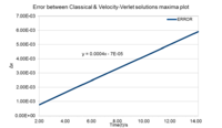
Task 2: Plot of maxima error positions vs time
The coordinates of the 5 maximas in figure 2 were estimated and plotted on a new graph. This yielded a linear function where
.
Task 3: Timesteps to minimise variation in total energy
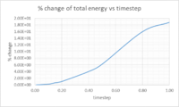
Multiple timesteps were used to calculate the total energy of the harmonic oscillator. The percentage difference was taken between the initial energy assumed to be correct and the energy of the first minima, these results were then plotted(figure 3). In order to keep the change in total energy below 1% a timestep equal to or below 0.2 should be used. The change in total energy of the simulation should be kept to a minimum as the total energy should not vary over time in the harmonic oscillator.
Task 4: Lennard-Jones interaction
1. Calculation of distance at zero-potential, r = r0:
where φ = potential energy r = the distance ε = well depth and σ = distance from zero potential distance
2. Force at r0:
Since
3. Finding the equilibrium separation req:
4. Finding the well-depth at equilibrium:
5. Evaluation of integrals:
a)
b)
c)
Task 5: Estimating the number of molecules in volumes of H2O
1. Number of molecules in 1mL:
2. Volume of 1000 molecules:
Task 6: Periodic boundary conditions
When the atom at in the cubic simulation box to moves along the vector it ends up at (when the periodic boundry condition is taken into consideration).
Task 7: Converting reduced values to real values:
1. Reduced distance
2. Well-depth
3. Temperature
Equilibration
Task 8: Problems with random starting coordinates in non-solid simulations
If atoms were given random starting coordinates then they could end up within a contact proximity, they could bump into each other and then they would not only experience the potential of each but also the kinetic energy.
Task 9: The number density of lattice points calculations:
The number density n is given by the following equation
where N is the number of atoms/lattice points per unit cell and V is volumes of the unit cell.
1. The number density of a simple cubic lattice with inter lattice point distance of 1.07722
For a simple cubic lattice there is one atom/lattice point, therefore;
2. Side length of a face-centred cubic lattice with a number density of 1.2
A face-centred cubic lattice has 4 atoms/lattice points, therfore;
Task 10: How many atoms are created by create_atoms 1 box command for a face-centred cubic lattice?
Since there are 4 atoms per lattice and the box is ten lattice spacings larger than the single lattice spacing then there would be 4000 atoms.
Task 11: LAMMPS commands for setting the properties of atoms:
1. Mass command
mass I value = mass 1 1.0
This command is used for setting the mass of the atom, in the general command I is the atom type and value is the mass(in reduced units). In the example the atom is type 1 and the mass is 1.0.
2. Pair_style command
pair_style style args = pair_style lj/cut 3.0
The pair_style command is used to describe paired interactions, style is the interaction which is being looked at and args is the argument used for that style. In the example above the style is defining the cutoff distance, that is the distance at which interactions become negligible. The argument for the cutoff distance is 3.0, after which the simulation will not compute.
3. pair_coeff command
pair_coeff * * args = pair_coeff * * 1.0 1.0 This command is used to define the force field coefficients between pairs of atoms, the asterix terms are to define the coefficients for all atoms, the second part of this command, args, defines the coeffecients.
Task 12: Specifying the velocity of each atom
The Velocity-Verlet algorithm is used to specify velocity and position
Task 13: Running the simulation:
The command $(100/timestep) command allows for the immediate evaluation of the the formula with the pre-defined variable i.e. the timestep. The following line variable n_steps equal floor(100/$({timestep}) will be broken down into individual contributions. The variable component is used to allows for the return to re-run a command, this allows creates a loop. The n_steps part describes the number of timesteps you wish to calculate which is defined in the 'Run Simulation' command. Equal is used to create a mathematical argument. Floor(11/$({timestep}) is useful in setting the maximum timestep bigger than the original one. In the run simulation part first we define the number of timesteps to be considered and then report the floor value i.e. the total time it takes. These lines are essential in creating a loop where each new timestep may be calculated subsequently. Make it easier to change the timestep, all values dependedent on the timestep will be changed with it and so it reduces possible human errors when changing all variables and also makes it easier and faster.
SPECIFY TIMESTEP variable timestep equal 0.001 variable n_steps equal floor(100/${timestep}) variable n_steps equal floor(100/0.001) timestep ${timestep} timestep 0.001
RUN SIMULATION run ${n_steps} run 100000
Task 14: Checking equilibration
1. Pressure, Temperature and energy against time for simulation ran at 0.001 timestep

2. Equilibration
The simulation reaches equilibration at approximately 0.28, this is the timestep at which the simulation becomes relatively constant.
3. Maximising results accuracy whilst keeping the timestep within a reasonable timescale
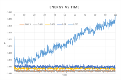
The best timestep for maximum accuracy and sufficient information is 0.0025. It overlaps with 0.001 and so although it is more than twice the time as 0.001 it maintains a satisfactory level of accuracy. The others give equilibrium energies which are too far off the most accurate value, with the worst being for 0.01 as it diverges quite dramatically.
Running simulations under specific conditions
Task 15: Finding the expression for factor
is a factor by which the velocity can be corrected.
(1) (2)
Where T' is the target temperature and T is the instantaneous temperature
Insert v_i into equation x
Task 16: The importance of number, repetition and frequency of average calculations with timesteps
fix aves all ave/time 100 1000 100000 v_dens v_temp v_press v_dens2 v_temp2 v_press2
100 sets the number of timesteps after which another thermodynamic value is used to calculate the average, 1000 is the number of thermodynamic values which are used for the average and 1000000 sets the frequency at which averages are calculated.
100000 timesteps will be run.
Task 17: Equation of state plots
5 temperatures above the critical temeperature were chosen(1.6, 1.8, 2.0, 3.0 and 5.0) these were all simulated with a pressure of 2.6(n-1) and also 3.3(n-2). The timestep chose was 0.01 as in previous experiments it was the largest timesteps yielding the most accuracy. The pressures were plotted against the temperatures along with their error bars.
The ideal gas densities were calculated with the following equation: where K_B = 1 in reduced terms
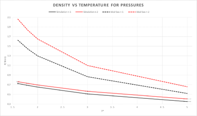
The simulated density is lower than that of the ideal gas method, this can be explained by an assumption to satisy an ideal gas. The atoms must not have any forces upon them and also they mustn't take up any space. In the simulation the atoms do take up space and therefore they have a lower density. This discrepancy increases with pressure. The general trend of the two plots is a decrease in heat capacity as temperature is increased.
Heat Capacity Calculation
Task 18: The temperature dependence of the isochoric heat capacity
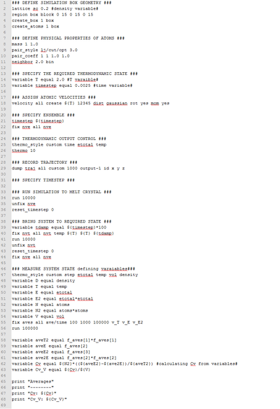
A LAAMPS script which could calculate the isochoric heat capacity from calculated thermodynamic values was used figure 7. The Cv/V was calculated with the following equation;
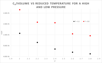
The effect on heat capacity at different temperatures and pressures
The decrease in heat capacity at higher temperatures is a result of the non-classical behaviour of the system at low temperatures. The energy levels behave as if they are discrete, the lower the temperature the more discrete they are. As illustrated here, the energy levels are closer together at higher temperatures e.g. and further apart at lower temperatures e.g.. When a heat increment, , is introduced into the two systems we see that it has a different effect in both. At , will give a greater temperature increase than , this causes the denominator in the equation below to become more important thus decreasing the isochoric heat capacity.
The difference between the two pressured systems in figure 7 is what would be expected, the higher pressure plot has a higher isochoric heat capacity. At a higher pressure the atoms are closer together, they can thus transfer heat more effectively with a given temperature change than a system with a lower pressure, since the atoms are further apart.
Structural properties and the radial distribution function
Task 18: The Radial Distribution Functions of a solid, liquid and gas
1. Comparisons of the solid, liquid and gas radial distributions functions as well as the integrated function
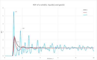
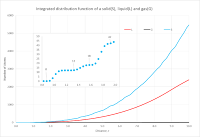
The distribution plot(figure 9) of the gas has one short, broad peak which is close to the reference atom; as you move further away the distribution becomes constant. This characteristic shows the small probability of finding an atom close to the reference atom; also when it becomes constant this shows how there is negligible probability of finding another atom at the distance studied. When looking at the integrated function(figure 10), it emphasizes how few atoms you will find in the distance, this is characteristic of a gas' dispersed atoms.
The liquid's distribution has a taller first peak than the gas' and then multiple peaks tapering off as you move further away; it is evident that there is a higher probability of finding an atom throughout the space than in a gas. Additionally the integrated distribution(figure 10) shows a larger number of atoms as you move through the space. This demonstrates the higher proximity of the atoms in the liquid state.
Finally the solid's distribution has a very sharp and tall peak close to the reference atom but then as you move further away the peaks become smaller but continuously fluctuate. The sharpness of the peaks and their continuous distribution arise from the highly ordered structure of the solid. The peaks are sharp unlike the gas and liquid because all of the atoms are in fixed positions and so at a certain position there will be a number of atoms in an equivalent position around the sphere of the distribution function. Furthermore the solid's first peak is considerably larger than the other phases, the probability is much greater due to the closeness of the atoms. The integrated function shows a very large number of atoms in the space, this again illustrates the closeness of the atoms in the solid state.
2. Using the solid RDF to extract information on the lattice structure
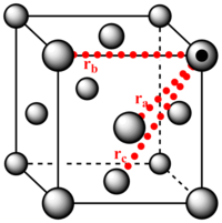
The three first peaks of the solid's radial distribution function are distances 1.0, 1.5 and 1.8. The lattice spacing is 1.5 and the calculated distances , and (where is the distance from the reference atom to the atoms a, b and c) were found to be 1.0, 1.5 and 1.8(respectively). Therefore the first three peaks 1, 2 and 3 correspond to the lattice points a, b and c(respectively).
The coordination of atom a, b and c is 12, 6 and 24(respectively). These values were interpolated from the magnification of the integrated solid distribution function.
Dynamical properties and the diffusion coefficient
Task 19: The mean squared displacement(MSD) of large and small simulations

where; the initial timestep and the new timestep.
The mean squared displacement(equation above) is a measure of how much random motion there is within the system. In this simulation the ability to move randomly is determined by the amount of free space and therefore the density. In the gaseous phase there is a lot of free space, the atoms move freely and encounter only a small number of atoms to collide with thus impeding it's motion; the linear increase of the plot reflects this behavior. The liquid has a lower degree of random motion than the gas, due closer proximity of the atoms, forces such as drag will now effect the atom's motion as it moves past other atoms. The two first plots show that the atom is able to move in drift, however the liquid experiences more drag and has a smaller gradient. The solid displays the least amount of translational freedom, the close packed structure prevents any random translational motion; it does however show some random movement, arising from vibrations of the constrained atoms. Therefore the plots in figure 12 are a reasonable representation of the random movement of the three phases.
Finding the diffusion coefficient
where the diffusion coefficient in , MSD and timestep The gradient of the slopes give the diffusion coefficient, however this uses a dimensionless timestep denominator, therefore we must convert it to time units by dividing by the timestep(0.002).
The gradient was found by fitting a linear trendline through the function.
Solid
Conversion of the gradient to give time units gave for the million atom simulation and for the 3200 atom simulation.
Liquid
Conversion of the gradient to give time units gave for the million atom simulation and for the 3200 atom simulation.
Gas
A trendline was fitted to the function, since the simulation took some time to produce the linear behavior it was fitted to be linear with the latter part of the function. Conversion of the gradient to give time units gave for the million atom simulation and for the 3200 atom simulation.
Task 20: The velocity auto-correlation function(VACF)
Evaluating the 1D harmonic oscillator VACF using the expression for the position as a function of time
The normalized VACF is given by;
We must simplify this expression in order for it to be useful, to do this we must first find expressions for and :
The expression for position as a function of time for the HO is defined as;
This can be substituted into the expression of velocity as a function of time;
This is then differentiated using the chain rule;
Where
We also need our velocity as a function of time after , this is acheived by substituting in ;
The two velocity expressions are substituted into the VACF;
Using the trigonometric identity we can re-write our equation;
where and
The fraction can be expanded;
Then since does not contain a t term it can be moved outside of the integral;
The alike terms cancel to give;
Finally , this is because and are odd functions. When odd functions are integrated between symmetrical boundaries the product is zero.
Therefore;
Analysis of the Lennard-Jones(LJ) solid, liquid and harmonic osillator(HO) VACFs against position
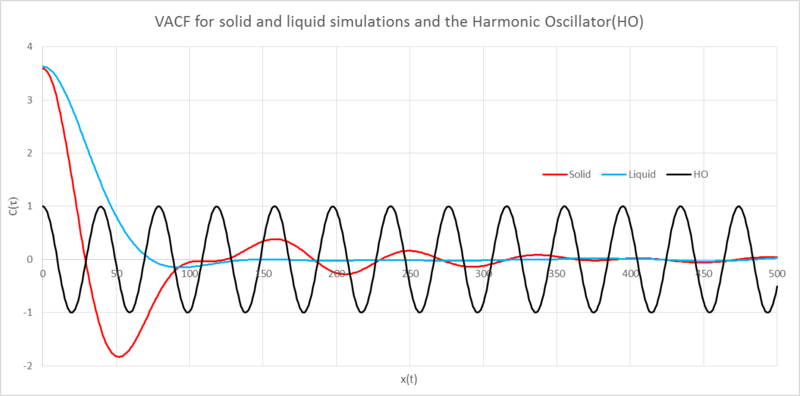
The minima in the VACFs represent a change in the direction of the velocity, this caused by collisions with other atoms.
The liquid and solid VACFs are similar but have some important differences. The solid VACF reaches its minima much quicker than the liquid; the atoms in the solid are much closer together and so have more surrounding atoms, it therefore takes less time for atoms to collide. The decorrelated solid function shows some oscillation about this arises from the jostling about with other atoms in the fixed lattice and so we see a sort of harmonic oscillator motion. The liquid does not display this behaviour because they are free to move and so will be able to "rapidly destroy any oscillatory motion."[1] by the "diffusive motion".
The LJ VACFs become decorrelated after colliding with other atoms, after collision the subsequent velocities no longer depend on the initial velocity. The Harmonic Oscillator’s VACF is fully correlated with the initial velocity. It behaves periodically, always returning through the same points after a certain amount of time. The differences seen between these plots are rooted in the essence of the representations. The HO models two sphere’s connected by a spring, the spring may expand and contract with perfect elasticity. In addition to this there are no external forces which could cause the velocities to decorelate. The LJ representions are effected by surrounding atoms, the velocities loose their correlation after a collision.
Task 19: Integrating using the trapezium rule to get D
The plots of of the three phases in a small and large system were plotted along with their running integral.
The first part of this equation is the relationship between , the diffusion coefficient and the VACF. The second part is the equation used in excel to calculate the running integral. Where is the velocity, is the timestep and is the last integral calculated. The last value of the running integral was divided by 3 to give .
Solid(figures 14-15)

for the small solid simulation and for the million atom simulation.

Liquid(figures 16-17)
[[File:liquid8000.png|200px|thumb|left|figure 16 VACF and running integral vs time for 8000 atom liquid simulation] for the small liquid simulation and for the million atom simulation.

Gas(figures 18-19)

for the small gas simulation and
for the million atom simulation.

The diffusion coefficients are as would be expected for the respective states. An atom in a tight lattice is not free to diffuse and is locked in position, this is reflected in its very small value. The liquid has a more important diffusion coefficient since the atoms are free to move, however they do experience more impeding forces such as drag while passing other moving atoms. Finally the gas is also a reasonable estimation, it is much greater than the solid and liquid since the atoms are a lot more disperse and so move very quickly and encountering relatively few restrictive forces.
Sources of error in the estimates
A larger number of atoms included in the simulation gives a more accurate result, therefore the million atom simulation and the smaller one do have a small difference in values which can be accounted for by this. Another important source of error comes from the running integral calculation, each new area will have the previous area added to it, this results in a build-up of errors. The two solid diffusion coefficients calculated from the running integral are an order larger than the coefficient calculated using the mean squared displacement method.
References:
