Rep:Mod:HB2515MgO

Abstract

The thermal expansion coefficient of MgO was calculated using DLVisualize and GULP, which simulate the properties of the crystal lattice structure. Two different techniques which have different approximations and assumptions were used: Lattice dynamics and Molecular dynamics. It was found that lattice dynamics achieve more accurate solutions in comparison to molecular dynamics, but the results from both techniques were very close. The thermal expansions calculated were 3.0 x10^-5 K^-1 and 2.9 x10^-5 K^-1 for lattice and molecular dynamics respectively, compared to lit. which is found to be 4.0 x10^-5 K^-1 from 300-1200 K .

Introduction

Importance of modelling

Vibrations in a solid can be used to predict the materials behavior, notably when heated (such as thermal expansion), or other properties being phase transitions, transports, electrical properties and dielectric phenomena for example.

To get an idea about the potential applications of these materials, computational chemistry is used to model atomic motion using different approximations, before calculating and predicting more properties. The different materials can then go on to be used in creating new devices, which take advantage of the displayed characteristics.

Sensors which trigger lights to switch on automatically illustrate this idea nicely. Inside one of these sensors is a crystal of Wurzite (ZnO) which has pyroelectric properties. These properties cause a change in net polarisation upon a change in temperature, which is communicated to the device, triggering the light. This is in fact more delicate than it sounds, as it is important that the light only switches on for human movement to limit the energy waste. By studying pyroelectric materials, and their anisotropic thermal expansion, through making small changes to their composition, whilst computationally modelling them to get the exact interval of radiation absorbed by it, it is possible to create such products.

To study the theory behind thermal expansion, computer software is used to model the behavior of the crystal structure and calculate the variations of different parameters. From this data, many different properties can be calculated and compared to the values obtained practically in the lab. Different approximations (some more accurate than others) are used to do this modelling which will be demonstrated in this study where the lattice dynamics and molecular dynamics are used and contrasted.

Lattice dynamics

When performing calculations on the lattice of the crystal structure, Quasi-Harmonic Approximation (QHA) is used. This approximation differs from the Harmonic approximation (HA) only by considering that the frequency is dependent on the volume of the crystal considered in QHA.

As for any atom in a structure, it vibrates around an equilibrium position. These vibrations can be modeled classically or quantum mechanically. In HA and therefore QHA, these vibrations are thought of quantum mechanically. The sum over all the atoms is then taken using a Taylor series, giving the energy total energy of a crystal. All the terms above the cubic polynomial are ignored, which leads to the approximation that the crystal is a combination of lots of small harmonic oscillators. In this model, the vibrations of each atom are not independent, meaning that the vibrations travels through the material, giving rise to a harmonic travelling waves . In the same fashion that electromagnetic waves are quantised and named photons, these vibrational waves are called phonons.

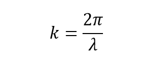
Phonons are not represented in real space, but rather in k-space (or reciprocal space). The k wavevectors gives information about their momentum and their direction, related to the wavelength as:

(equation 1)

In real space, one of the parameters of the periodic cell examined is a. In this reciprocal space, the equivalent is a* and is related to a as:

(equation 2)

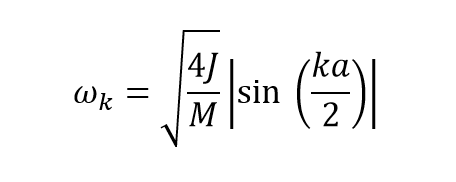
The wavevector varies in the interval -π/a to π/a which is also known as the first brouillon zone. This wavevector can be plotted against the frequency to give a phonon dispersion curve using

(equation 3)

This was found to be a good approximation, but it doesn't work for high temperature, as it doesn't take into account unharmonic interactions. Just like the harmonic oscillator which is only a good model for bonds vibrating very close to their equilibrium, as the energy increases, the approximation becomes worse. In this model, it doesn't predict the bond to ever dissociate, but it is a known fact that at high temperature, materials decompose.

Molecular Dynamics

The principle of molecular dynamics is to use classical physics to model the particles in the material. The charges are distributes, and the movement of these ions are calculated computationally by solving Newtons second law of motion. A timestep is selected and at every timestep the calculation are run based on the new positions and velocities of the ions. This is done until an equilibrium is reached, when the program will stop running and return the results. This is a good way of modelling higher temperatures, as it was seen that this was difficult using lattice dynamics.

The limitation to molecular dynamics is that the computational processing power is much larger than the previous method, meaning that the calculations take a long time to run, and sometimes can even be processed at all. It was also observed that this approximation is not very accurate for low temperatures.

The aim of the model

By using the 2 different models, the aim is to determine the volume of the conventional cell in an MgO crystal structure. Using this data, the lattice constants may be calculated and plotted. This curve can be extrapolated and used to find the thermal expansion coefficient.

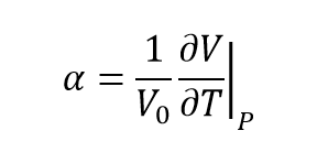
To find the thermal expansion coefficient, the following equation is used:

(equation 4)

Method, Results and discussion

Structures used:

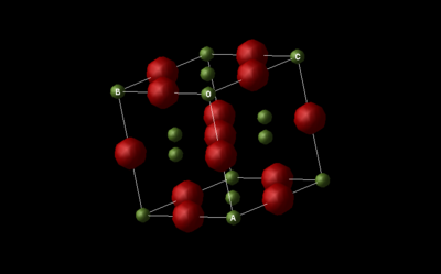
For the Mgo crystal structure, two different types of unit cells exist: the primitive unit cell which is a rhombohedron with an internal angle of 60 degrees and contains 1 Mg atom and 1 O atom, or a conventional unit cell, which is 4 times the volume of the primitive unit cell, containing 4 Mg atoms and 4 O atoms. The conventional unit cell is face centered cubic (fcc) and better represents the crystal structure, which is why it is more widely used when for describing the lattice of MgO. These two cells both have the same density, which means that inter-converting between them is just a question of multiplying by 4. This is interesting when performing computational calculations, as it is possible to perform the calculations on the primitive unit cell (smaller therefore easier and faster to process) before converting the results to the conventional unit cell.

Figure 1: Primitive unit cell of MgO	Figure 2: Conventional unit cell of MgO

Lattice dynamics:

Phonon Dispersion and Density of States

A phonon dispersion curve is a was of plotting the variation in frequency at all the different k values in reciprocal space. As the crystal has 3 dimensions, we will have k values in all of those three dimensions, therefore kx, ky and kz. When plotting this we encounter the problem that the plot will have to be 4D, which is not possible. Potentially a 3D plot with a colour code could replace this and be a temporary solution to the problem, but this is not the best general solution. To solve this problem, kx, ky and kz will all vary to different values varying from -π/2 to π/2 (first brouillon zone) whilst describing the frequency for every phonon mode at each set of k values. The number of normal mode here is 3N with N the number of atoms. The translation and rotation of the periodic lattice are the reason it is not 3N - 6 as for usual molecules.

In the equation above, a and a* are inversely proportional. Therefore if the unit cell in real space is smaller (smaller parameter a), the reciprocal space will be larger, and it may require more calculations and data points to get accurate results (calculating more wavevectors k).

The phonon dispersion plot give a relationship between the frequency and the wavevector k. While computing the phonon dispersion curve, 50 different wavevectors were calculated giving a plot as follows:

Figure 3: Phonon dispersion plot for 1x1x1 grid size

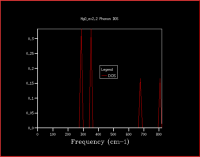
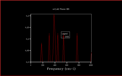
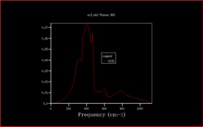
It is then possible to generate a density of states diagram, by summer over all the different states for a particular frequency, but only one wavevector. This is represented by the following plot with is for a 1x1x1 cubic cell.

Figure 4: Density of states (DOS) for 1x1x1 grid size

These vibrations gives sharp peaks at precise frequencies. We should be expecting 6 different normal modes, as mentioned previously. This is what we observe in fig. 4, but some peaks are overlapping and we observe the integration in a 2:2:1:1 ratio. Therefore we can identify that this corresponds to the set of wavevectors at the L point from the dispersion plot by comparing with the number of branches at that point in the dispersion plot. This can be checked by examining the output file which confirms the ratio that was suspected, labeling the acoustic modes give peaks at 286 and 351 cm-1 and 0.333 and the optical modes give peaks at 676 and 806 cm-1 as 0.167. The two acoustic peaks are both doubly degenerate. The log file also reinforces this by examining the frequencies at point L matching the density of states plot at (0.5, 0.5, 0.5).

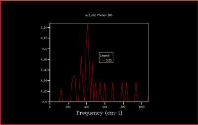
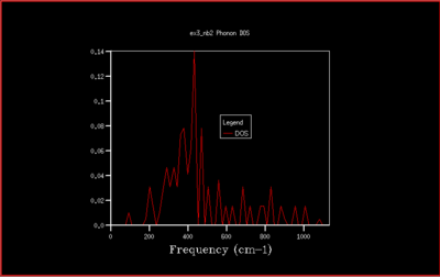
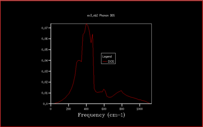
This is not however a good representation of reality because a crystal is formed of a infinite number of cells next to each other arranged periodically. To increase the grid size, larger shrinking factors are selected, which will spread the frequency bands over a larger number of states in the DOS plot whilst increasing the number of wavevectors at which the frequency is calculated and displayed in the plot. Many different grid sizes were tested, and 40x40x40 was selected giving a smooth curve, whilst maintaining a realistic time per calculation.

Grid size and free energy

As mentioned before, by summing over all the states in the DOS plot, it is possible to obtain the free energy of the crystal. As the grid size increases, the accuracy of the energy also increases. As seen in the table below, the energy converges to 6 dp quite rapidly, and by a shrinking factor of 20 the differences in the values are too small to be recorded. This is also represented in the graph below (figure 5) which shows the free energy converging to the final value, gaining in accuracy. As seen in the table below (table 1) to get an energy accurate to 1 meV, a grid size of at least 2x2x2 could be used, for an accuracy of 0.5 meV a grid size of at least 4x4x4 is required, and finally, if the desired accuracy is of the 0.1 meV order, at least a 4x4x4 must be used.

Grid size	Free energy/eV	Difference from Converged value
1x1x1	-40.930301	0.003818
2x2x2	-40.926609	0.000126
3x3x3	-40.926432	0.000051
4x4x4	-40.926450	0.000033
10x10x10	-40.926480	0.000003
15x15x15	-40.926482	0.000001
20x20x20	-40.926483	0
30x30x30	-40.926483	0
40x40x40	-40.926483	0
50x50x50	-40.926483	0

Table 1ː Accuracy of energies for different shrinking factors

Figure 5: Plot showing energy values converging to more accurate value for higher grid sizes

In this study the binding energy of the crystal lattice of one unit cell was calculated and found to be -40.9303 eV. As the grid size increases, the density of states (DOS) is computed for a larger number of k-values and the plot becomes more accurate, converging to the ideal shape (for infinite grid size). Increasing the grid size beyond 40x40x40 only changes the density of states plot a little, and doesn't change the value of the free energy. Therefore the computational time would be much longer, and with no real benefit. The optimal shrinking factor was therefore selected as 40, at which the DOS plot is smooth and averaged out, whilst not being to long to compute using the software, giving a reasonable approximation. At this optimal grid size, the DOS is more accurate than smaller grid sizes, and a little less accurate than larger grid size but computationally slower, but computationally much faster. All the graph with the different grid sizes are shown below in Fig. 5-14:

Figure 6: MgO Density of states at 300K for grid size 1x1x1	Figure 7: MgO Density of states at 300K for grid size 2x2x2

Figure 8: MgO Density of states at 300K for grid size 3x3x3	Figure 9: MgO Density of states at 300K for grid size 4x4x4

Figure 10: MgO Density of states at 300K for grid size 10x10x10	Figure 11: MgO Density of states at 300K for grid size 15x15x15

Figure 12: MgO Density of states at 300K for grid size 20x20x20	Figure 13: MgO Density of states at 300K for grid size 30x30x30

Figure 14: MgO Density of states at 300K for grid size 40x40x40	Figure 15: MgO Density of states at 300K for grid size 50x50x50

As mentioned previously, the grid size is dependent on the the size of the reciprocal space, therefore the brouillon zone. Due to the inverse proportionality, if the lattice constant (a) is larger, the reciprocal space constant (a*) will be smaller, and a smaller grid size will be enough to achieve the same accuracy. The opposite is also true.

So when looking at a crystal of CaO , which has a lattice parameter of a=4.811 Å , compared to a=4.21 Å for MgO and has the same structure (fcc, high in symmetry), the same grid size would be applicable to CaO. The symmetry is key also, as the program will recognise this and perform less calculation, by just applying the same results by symmetry.

In the case of the Zeolite Faujasite, the lattice constant a is much larger as the molecule is a large complex framework. It is found in literature to be anywhere between a=24 Å and a=26 Å . With the same logic as previously applied, a much smaller grid may be use for the zeolite.

Finally in the case of a metal such as Li, a=3.5092 Å , a larger grid would be required. This smaller lattice constant is the result of metallic bonding and small Li ions, with very strong and hard charges.

Free energy and lattice contant:

Figure 16: Helmholtz free energy as the temperature increases

In Fig. 16, the Helmholtz free energy is plotted in function of the temperature, varying from 0 to 2900 K. The equation relating the free energy and temperature is:

(equation 5)

The graph is decreasing as T increases due to the entropy term becoming more dominant as the temperature increases (because -TS). In the graph, at high temperature the line becomes straight. This would mean that at low temperature, the internal energy U and entropy S are still weighting on the free energy term. But when T is very large, the change in U and S is not important enough compared to the change in temperature, meaning that the graph takes a y=mx+p shape with a negative gradient. This is due to the fact that the quantum mechanical approximations using QHA take into account the zero-point energy.

Figure 17: Lattice constant of MgO crystal structure variation with temperature using the 2 approximations

The lattice volume was also recorded for the same temperature interval, and is plotted above (Fig. 17). To find this value, simple calculation were performed, converting the volume of the primitive unit cell in the output file to the volume of the conventional unit cell (multiplying by 4) to give the result. The volume was then cube rooted to give the lattice constants. As expected, as the temperature increases, the average volume of the unit cell increases, increasing the lattice constant (the cubic root function is positive and increasing, this means is does not affect the variation of the function over the interval). This is because the atoms are vibrating the a greater extent, taking up on average a greater volume per atom. As observed above, the unit cell continues increasing in volume even when the temperature is very high, and this is where the methods does not provide a good approximation anymore. At this high temperature the bonds should breaks, however this is not taken into account in the QHA, which does not take into account anharmonincity.

Thermal expansion coefficient

From the equation:

(equation 6)

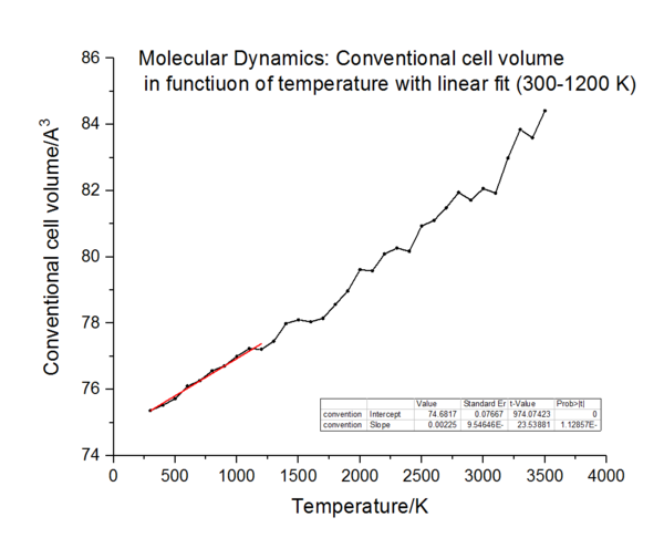
can be extrapolated the expansion coefficient. The conventional cell volume is plotted against the temperature to show the variation of this volume with temperature, which will be extrapolated to get the gradient to use in equation 6. Both approximations are used to find this in the two curves below:

Figure 18: Conventional cell volume change with temperature using lattice dynamics

Figure 19: Conventional cell volume change with temperature using molecular dynamics

The linear part of these curves is fitted and the slope is extracted over the temperature 300-1200 K. From this slope, using the previous equation, the thermal expansion coefficient is calculated and the results are as followed:

For the Quasi-Harmonic approximation, the coefficient of thermal expansion is calculated to be 3.0 x10^-5 K^-1 (lit. 4.0 x10^-5 K^-1 from 300-1200 K) For molecular dynamics 2.99 x10^-5 K^-1.

Comparing the 2 methods:

Both lattice and molecular dynamics have given very similar results. They are close to the values obtained experimentally with a percentage error of 25%. This value is close to the one observed experimentally. Models like this are very powerful at predicting theoretical values like this.

For the lattice dynamics the main approximations as mentioned earlier are the fact that all the molecules vibration in a harmonic fashion and that arhomonicity is never reached even at very high temperature. This means that at lower temperature the value should predict a value close to the one found experimentally, which it has done. Furthermore, as this method takes into account zero point energy, it should be able to predict these properties at low temperature. In literature, the thermal expansion coefficient is found to be 1.0 x10^-5 K^-1 between 0-300 K. The curve is not a straight line in this plot and it can be seen qualitatively that the gradient is reduced for this approximation between 0 and 300 K. This would result in a lower thermal expansion coefficient just like literature. However it would be necessary to perform a larger number of calculations in that interval to get a reliable result.

For the molecular dynamics, the main assumption is that all the physical interactions are classical. This theory predict the breakdown of the material which is an advantage, but completely ignores the quantum mechanical affects such as zero point energy. As it can be seen on the graph, the straight line fitted between 300-1200 K can be carried on all the way down to zero. This would predict an identical thermal expansion coefficient for that region, which is not the case as mentioned when discussion the lattice dynamics (it is in fact . 1.0 x10^-5 K^-1 between 0-300 K).Therefore, this model does not work as well for lower temperature.

In the same logic, if the temperature range was selected differently, the two models would give different results, with the molecular dynamics predicting higher temperature more accurately, and the lattice dynamics representing a good model at lower temperatures. At very high temperature (past the melting point), the theories should collapse.

As the temperature approaches the melting point (3125 K), the approximation should break down. This is clearly observed on the molecular dynamics plot, where the point start to scatter and don't remain in a straight line. Therefore the phonons do not represent the actual motion of the ions very well anymore.

Resulting from all this, using QHA at very high temperature would give very large volumes of conventional unit cells, and MD would predict that the bonds would break, therefore there would not be any unit cells.

In a diatomic, when the temperature is increased, the molecule vibrates more, stretching its bond even further, and the kinetic energy from the heat supplies more energy to be converted into potential energy in the spring-like bond between the two atoms. This means the molecule spends a greater deal of time at larger bond length, therefore increasing the average bond length. In other word, the bond length simply increases when heated. The same is happening in the Mgo crystal structure, which is perceived as the increase in the cell volume. This is because use the QHA, the material is formed of lots of small harmonic oscillators as mentioned previously.

Experimental

The calculations for this study were performed on a General Utility Lattice Program (GULP) and represented in 3D in the DLVisualise interface in the Linux environment. For all calculations, a conventional cell of the crystal structure of MgO was uploaded unless indicated otherwise and the energy calculation was performed without including the shells in the select potentials panel and the ionic.lib was selected.

Phonon modes

Calculation of the internal energy of MgO:

In the GULP panel, single point was selected. After running the calculations, the energy was found to be -3963.1403 kJ/mol cubic cell.

Calculating the phonon modes of MgO:

-Dispersion curves: The phonon modes of MgO were calculated using the software previously described. In the Execute GULP panel Phonon Dispersion mode was selected, setting Npoints to 50. The phonon eigenvectors were calculated.

-Density of states: In the GULP panel, phonon DOS was selected in the general options and the different density of states were plotted for grid sizes varying from 1x1x1 to 50x50x50.

Free enegry calculation:

In the GULP panel, phonon DOS was selected under the general options. The temperature was set to 300K and the grid size was varied from 1x1x1 to 50x50x50.

Thermal expansion of MgO using the Quasi-Harmonic approximation:

The GULP panel was set to optimisation and under optimisation options, optimise Gibbs free energy was selected. The phonon DOS was selected and the grid size was set to 40x40x40. The temperature was varied from 0 to 3000 K.

Thermal expansion of MgO using Molecular Dynamics:

A supercell of 32 MgO units was uploaded to perform these calculations. The GULP panel was set to molecular dynamics and under the MD options, the ensemble NPT was selected. The time step was set to 1.0 fs, the number of equilibration steps ad production steps were set to 500. The number of sampling steps and trajectory write steps were set to 5. The temperature was varied from 300 to 3500 K.

Conclusion

In this computational chemistry modelling study, two different models were used. The first, lattice dynamics which relies on quasi-harmonic approximation was found to be good at low temperatures. This is due to the fact that it is quantum mechanical and it incorporates important notions such as zero-point energy. However the limitation to this model is that as with harmonic approximation, it does not take into account unharmonic effects and cant predict when the material will breakdown. It simulates the atoms to continue vibrating more and more violently. This would be very difficult to use i the material was not actually very stable a higher temperatures. Secondly, molecular dynamics was used o simulate the behavior of the MgO lattice at different temperatures. This approximation was concluded to be a better approximation for higher temperatures. This is due to the fact that modeling higher temperature with classical physics is closer to reality and the properties can be calculated with a better representation of the atomic scale. however this model did not work well for lower temperature, due to the fact that this classical model ignore quantum principles such as thew zero-point energy. Both result however did give good and very similar results when calculating the thermal expansion of MgO between 300 ad 1200 K. The thermal expansion, which is caused by the atoms vibrating to a greater extent, making the solid take up more volume was found to have a coefficient of 3.0 x10^-5 K^-1 for both model with only 25̥% error.

References

- ↑ 1.0 1.1 Studies on Thermophysical Properties of CaO and MgO by ɣ-Ray Attenuation by A. S. Madhusudhaan Rao and K. Narender Journal of Thermodynamics Volume 2014, Article ID 123478, http://dx.doi.org/10.1155/2014/123478
- ↑ 2.0 2.1 2.2 2.3 1 B. D. Boruah, S. N. Majji, S. Nandi and A. Misra, , DOI:10.1039/c7nr08125a.
- ↑ 3.0 3.1 Harrison, N. M., Vibrations in Crystals, lecture 4
- ↑ 4.0 4.1 4.2 Dove, M.T., Introduction to Lattice Dynamics, Cambridge University Press, 1993
- ↑ Introduction to the theory of lattice dynamics M. T. Dove EDP Sciences, 2011 DOIː 10.1051/sfn/201112007
- ↑ On how different the quasi harmonic approximation works for two isostructural crystalsː Thermal properties of periclase and lime A. Erba, M. Shahrokhi, R. Moradian, and R. Dovesi The Journal of Chemical Physics 142, 0441144 (2015) httpsː//doi.org/10.1063/1.4906422
- ↑ Computational Chemistry of Solid State Materialsː A Guide for Materials by Richard Dronskowski ISBN-10ː 3-527-31410-2
- ↑ Magnesium oxide (MgO) crystal structure, lattice parameters, thermal expansion Subvolume B 'II-VI and I-VII Compounds; Semimagnetic Compounds' of Volume 41 'Semiconductors' of Landolt-Bornstein - Group III Condensed Matter DOIː 10.10007/10681719-206
- ↑ Catalysis and Zeolitesː Fundamentals and Applications J. Weitkamp, L. Puppe Springer-Verlag Berlin Heidelberg 1999 ISBNː 978-3-540-63650-2
- ↑ Lattice Constants of Seperated Lithium Isotopes by E. J. Covington, and D. J. Montgomery The Journal of Chemical Physics 27, 1030 (1957)
- ↑ 11.0 11.1 Anderson, O.L, Zou, K., Thermodynamic Functions and Properties of MgO at high compression and High temperature, Journal of physical and Chemical Reference Data, 1990, 19, pp 69
- ↑ Bornstein, R., Landolt., Semiconductorsː Semimagnetic Materials, Landolt-Bornstein Group III Condensed Matter, 2011, vol. 41B, pp 1-6