Rep:Mod:DS4113 CMP

The Ising model is a theoretical model used to examine variuos phenoma (e.g. ferromagnetism, activity of neurons in the brain,..) using statistical methods. The model was first proposed by Willhelm Lenz back in 1920, and its 1D version was first analytically solved in 1925 by Ernst Ising. 2D version of this model was analytically solved by Larse Onsager in 1944, although his solution is only valid for $H=0$.

The model

In the model, spins (that can only be one of the two states, +1 and -1) are arranged into a lattice. Each spin can only interact with its nearest neighbours, and this interaction is the only contribution to the energy of the system.

So we can write: $$\begin{gathered} E=-\frac{1}{2}J\sum _i^N\sum _{j \\ \in \\ \mathrm{n}\mathrm{e}\mathrm{i}\mathrm{g}\mathrm{h}\mathrm{b}\mathrm{o}\mathrm{u}\mathrm{r}\mathrm{s}\left(i\right)}{s}_i{s}_j \end{gathered}$$ , where $J$ is an interaction constant.

J can either be:

• Positive: we are dealing with a ferromagnetic material

• Negative: we are dealing with an  antiferromagnetic material

• Zero: spins are not interacting

Lowest energy

It can be shown that the lowest possible energy for the Ising model $E=-JND$, where $J$ is the interaction constant, $N$ is the number of particles / spins, and $D$ is the dimensionality of the lattice:

1. Assume that at lowest E, all the spins are aligned.
2. In 1D, there are 2 sites of contact for each lattice; in 2D, there are 4 sites of contact; in 3D, we have 6 sites contact,… Generally, for D-dimensional system, there are going to be 2D sites of contact. From this fact, we can deduce that $E\propto 2D$  .
3. That means that $$\begin{gathered} \sum _{j \\ \in \\ \mathrm{n}\mathrm{e}\mathrm{i}\mathrm{g}\mathrm{h}\mathrm{b}\mathrm{o}\mathrm{u}\mathrm{r}\mathrm{s}\left(i\right)}{s}_i{s}_j=2D \end{gathered}$$ as for a lattice with all spins aligned,  $s_i{s}_j=1$, and there is a total number of 2D interactions for each spin.
4. Now, as there is $N$ spins, each experiencing the same interaction energy, $E=2D$.
5. Simply substituting the above result to the full equation, we can deduce that $E(min)=-JND$ .

At this state of all spins being aligned, the multiplicity of the system is zero, meaning the entropy of the system is also zero.

Ising model was one of the first theoretical models to show a phase transition. This was a very important result back in early 20^th century, as scientists were still unsure whether the atomic theory can describe phase transition fenomena.

Curie temperature

It is the balance between the system’s energy and entropy that governs the behaviour of the system. From the 3^rd Law of thermodynamics, we know that that as the temperature approaches 0 (K), the entropy approaches 0 (J/(K.mol)). Therefore, we can expect that at lower energies, the behaviour of the system will be dominated by the energetic part, and the system (its spins) will be ordered. As the temperature increases, the entropic effects take on, and at large temperatures, the spins will be oriented randomly. The temperature at which the transition between these two states occurs is called the Curie temperature.

Let’s explore this behaviour more quantitatively. We have a 3D system with N = 1000. How does the entropy and the energy of that system change after randomly flipping one of the spins?

1. As each spin can only interact with its neighbours, we can calculate the internal energy of the system after spin flip as the energy of the system with all spin aligned + the destabilising interaction due to the flipped spin.
2. So we can write: $E=E(min)+E(interactions)=-JND+6*E(singleinteraction)=-JND+6*J=-J*1000*3+6J=-2994J$

Fig. 1. The magnetisation of both the 1D and 2D system is 1.

How about the entropy?

1. Bolzmann’s formula for entropy is $S=k_B\ln W$

1. In our case $S=k_B\ln (\genfrac{}{}{0ex}{}{1000}{999})=k_B\ln 1000\approx 10^{-22}J/K$

We can see that even after multiplying this with the number of particles, the entropy of this configuration is still very small compared to the energetic contribution.

Magnetisation

Another useful description of the state is its magnetisation, M. To omit the size of the system, we can also define magnetisation per spin.

$M=\sum _i{s}_i$

We can therefore expect the magnetisation per spin to be ±1 at low temperature (for example, at absolute zero, the magnetisation of a 3D system with N = 1000 would be ±1000), and reaching zero at high temperatures.

As mentioned previously, the analytical solution (for H = 0) was found by Onsager. The solution can be found here. In the rest part of this article, we will try to confirm his solution computationally.

Computational set-up

First of all, we have to create a random lattice of n X n spins:

def __init__(self, n_rows, n_cols):         self.n_rows = n_rows         self.n_cols = n_cols         self.lattice = np.random.choice([-1,1], size=(n_rows, n_cols))

To calculate the energy and magnetisation of this random lattice, we define energy(self) and magnetisations(self) functions:

def magnetisation(self):         return sum(map(sum, self.lattice))/1.0

The magnetisation can be simply calculated as a sum over the rows and to columns of the lattice. The result is divided  by 1.0 to ensure that ty result is a float.

The energy can be calculated by summing over each element of the lattice:

def energy(self):         energy = 0.0         for i in range(self.n_rows):             for j in range(self.n_cols):                 S = self.lattice[i,j]                 WF = self.lattice[(i+1)%self.n_rows, j] + self.lattice[i,(j+1)%self.n_cols] + self.lattice[(i-1)%self.n_rows,j] + self.lattice[i,(j-1)%self.n_cols]                 energy += -(WF)*S         return energy/2.0

This code is, however, very time-consuming. To make the code more effective (and perhaps more elegant?), we are going to replace the step-by-step process using Numpy roll and multiply functions. Numpy roll function can move the entries in our lattice. More about the function can be found here. For our energy calculations, we will simply:

1. Create a new lattice by moving the rows ‘up’ by one.
2. Create a new lattice by moving the rows ‘down’ by one.
3. Create a new lattice by moving the columns ‘left’ by one.
4. Create a new lattice by moving the columns ‘right’ by one.
5. Sum these 4 new lattices.
6. Multiply by our original lattice.
7. Sum all the entries of the array.
8. Multiply by necessary constants.

This algorithm effectively calculates $$\begin{gathered} \sum _i^N\sum _{j \\ \in \\ \mathrm{n}\mathrm{e}\mathrm{i}\mathrm{g}\mathrm{h}\mathrm{b}\mathrm{o}\mathrm{u}\mathrm{r}\mathrm{s}\left(i\right)}{s}_i{s}_j \end{gathered}$$ in just a few steps.

def energy(self):faster_energy = 0.0         sum_of_neighbours = []         sum_of_neighbours.append(np.roll(self.lattice, 1, axis = 0) + np.roll(self.lattice, 1, axis = 1) + np.roll(self.lattice, -1, axis = 0) + np.roll(self.lattice, -1, axis = 1))         faster_energy = sum(np.multiply(self.lattice, sum_of_neighbours))         return -sum(sum(faster_energy))/2.0

To compare the effectiveness of these codes, we run 2000 Monte Carlo steps for a 25x25 lattice (more about this later) 10 times for each code, using following code:

import timeimport IsingLattice as il import itertools import numpy as np #use a relatively big lattice of 25x25 so that we get more accurate timing data n_rows = 25 n_cols = 25 MEAS = [] # MEAS array will keep the results of out trials lattice = il.IsingLattice(n_rows, n_cols) for _ in itertools.repeat(None, 10): #record the time at which we start running     start_time = time.clock()     #do 2000 monte carlo steps     for i in range(2000):         lattice.montecarlostep(1.0)     #record the time at which we stop running     end_time = time.clock() #work out how many seconds the loop took, and print it     elapsed_time = end_time - start_time      MEAS.append(elapsed_time)     average_time = np.mean(MEAS) stdev = np.std(MEAS) repeats = len(MEAS) print"Average time: {} s".format(average_time) print"Standard deviation {} s:".format(stdev) print"Number of repeats:".format(repeats)

It was found that the second code was almost 8 times faster! (9.084±0.110 s vs 1.120±0.042 s).

Now, to find a stable state at some particular temperature T, we are going to use two important methods:

1. Importance sampling
2. Monte Carlo method

Combining these two methods, we get a so-called Metropolis-Monte Carlo algorithm.

Metropolis-Monte Carlo algorithm

This algorithm helps us to find the stable state by:

1. Flipping random spins where it is energetically favourable. (energetic part)
2. If the flip would be unfavourable energetically, the algorithm compares the Bolzmann factor ($e^{-\mathrm{\Delta }E/kT}$) with a random number to determine whether to flip the spin, or not. As the temperature rises, the probability of random a spin-flip, even though energetically unfavourable, will be higher. (entropic part)

The whole algorithm can be found here.

To translate this algorithm into a code:

def montecarlostep(self, T):         energy = self.energy()         magnetisation = self.magnetisation()         I = np.random.choice(range(0, self.n_rows))         J = np.random.choice(range(0, self.n_cols))         #the following line will choose a random number in the rang e[0,1) for you         random_number = np.random.random()         n_cycles = 0         W = self.lattice[I,J]                 S = self.lattice[(I+1)%self.n_rows, J] + self.lattice[I,(J+1)%self.n_cols] + self.lattice[(I-1)%self.n_rows,J] + self.lattice[I,(J-1)%self.n_cols]           interaction = W*S         if interaction =< 0:             self.lattice[I][J]=-1*self.lattice[I][J]         elif interaction > 0 and random_number <= math.exp(-int(2*interaction)/T) :             self.lattice[I][J]=-1*self.lattice[I][J]         else:             self.lattice[I][J]=1*self.lattice[I][J]         energy = self.energy()         magnetisation = self.magnetisation()         return self.energy(), self.magnetisation()

As discussed previously, the energy difference between the old and the ‘flipped’ lattice can simply be calculated just by focusing on the flipped spin and its closest neighbours. To make the process even more straightforward, ‘interaction’ was defined. It sums the spins of neighbours of the chosen spin, and multiply by the spin number of the chosen spin itself. Flipping the spin will lower the energy if interaction < 0. Let’s look at simple example:

Interaction = (1)*(-1-1-1+1) = -2, this suggest that the flip will lower the energy. This result is what we expect, as spins ‘like’ to have neighbours with parallel spins, rather than anti-parallel.

The above code runs a single Metropolis-Monte Carlo step and returns the energy and magnetisation after the step is performed.

Now, we need to define a function that will keep the results of each single step:

Eapp = [] E2app = [] Mapp = [] M2app = [] energy_2 = 0.0 magnet_2 = 0.0

Here, Eapp, E2app, Mapp, and M2app are empty arrays that will keep the energies, energies squared, magnetisations, and squared magnetisations, respectively. We also define energy_2 and magnet_2 as float-type constants that we are going to use

to calculate the squares of energy and magnetisation respectively:

Fig. 2. Magnetisation/per spin and Energy/spin [$J$] as a function of Monte Carlo steps.

Eapp.append(energy)energy_2 = energy*energy E2app.append(energy_2) Mapp.append(magnetisation) magnet_2 = magnetisation*magnetisation M2app.append(magnet_2)

This result of this procedure can be seen in Fig. 2. One important thing to mentioned is that it takes the system a few steps to reach the equilibrium positon. We want to exclude these steps from Eapp, E2app, Mapp, and M2app, as they represent non-equilibrium conditions:

def statistics():         del Eapp[:AAA]         del E2app[:AAA]         del Mapp[:AAA]         del M2app[:AAA]         E = sum(Eapp)/len(Eapp)         E2 = sum(E2app)/len(E2app)         M = sum(Mapp)/len(Mapp)         M2 = sum(M2app)/len(M2app)         EXLEN = len(Eapp)         return E, E2, M, M2, EXLEN

where AAA is the number of steps we want to exclude (it has to be an int-type!). Generally, smaller lattices takes fewer steps to reach the equilibrium. As for the temperature dependence, higher temperatures result in fewer steps to reach the equilibrium. The function then takes our arrays and returns the averaged values of energy, energy squared, magnetisation, and magnetisation squared.

Fig. 3. Example of a semi-stable state. 8x8 lattice. $T=0.1J/k_B$.

Table showing approximate number of steps needed to reach the equilibrium state for various systems

Temperature (J/kB) | Size of the system (LxL)	8	10	20	50	100
1.0	1 000	45 000	80 000	140 000	140 000
2.0	less than 1000	10 000	60 000	100 000	100 000
4.0	less than 1000	10 000	30 000	30 000	30 000
6.0	less than 1000	1 000	10 000	10 000	10 000

It is expected that at temperatures bellow the Curie temperature, the system should spontaneously end up in in a state with <M> ≠ 0.

It should be noted that sometimes, the system can end up in a semi-stable state. The results should therefore be checked to be sensible. For example, when running the simulation at T = 0.1, we can expect the spin to be all aligned. Sometimes, however, we can get to a semi-stable state where the spins form up and down ‘strips’. These results, however interesting, should be excluded from our statistical work.

The effect of temperature

Fig. 4. Dependence of the energy [J] of a 8x8 system on temperature[J/kB].

ILtemperaturerange.py was used to run the Metropolis-Monte Carlo over a range of temperatures $0.5J/k_B$ to $5J/k_B$) for a variety of systems (2x2, 4x4, 8x8, 16x16, and 32x32). This was performed 5 times for each system to gather enough data for further error analysis. As an example, one of the results for a 8x8 system can be seen bellow (Fig. 4.).

We can see that at lower temperatures, the magnetisation of the system is almost one and the energy is low. As the temperature increases, the magnetisation lowers, and the energy rises. This behaviour is as expected and discussed above.

Fig. 5. Dependence of magnetisation on temperature [$J/k_B$]. 2x2 system in red. 4x4 system in blue. 8x8 system in yellow. 16x16 in green. 32x32 system in cyan.

Fig. 6. Dependence of energy [J] on temperature [$J/k_B$]. 2x2 system in red. 4x4 system in blue. 8x8 system in yellow. 16x16 in green. 32x32 system in cyan.

As mentioned above, the calculations were run for different systems, 5 times for each system, except for the 32x32 system, for which the calculation run for over an hour so only one calculation has been done due to time-management issues. It can be seen from Fig. 5 and Fig. 6 that as the size of the lattice increases, the transition between the ordered state and disordered state is more sharp and the spread on the results becomes much smaller, possibly allowing for more accurate results (smaller standard deviation). However, as the lattice becomes bigger, the time needed to do the calculations rises exponentially, so there is always going to be an interplay between computational power and the accuracy of the results. One can mention that that the results for the 16x16 and 32x32 are approximately the same, with sharp transitions and small spread (deviation) of data, and as the 16x16 takes much shorter time to analyse, we can conclude that with limited computational resources, 16x16 system would be the best choice.

Code used for plotting Fig. 6, the code for Fig.5 was analogous:

T2 = []; M2 = []; T4 = []; M4 = []; T8 = []; M8 = []; T16 = []; M16 = []; T32 = []; M32 = [] i = open('2x2_all','r') for line in i:     a, b, c, d, e = line.split(' ', 4)     T2.append(float(a))     ene = float(b)/4.0     M2.append(float(ene))    j = open('4x4_all','r') for line in j:     a, b, c, d, e = line.split(' ', 4)     T4.append(float(a))     ene = float(b)/16.0     M4.append(float(ene)) k = open('8x8_all','r') for line in k:     a, b, c, d, e = line.split(' ', 4)     T8.append(float(a))     ene = float(b)/64.0     M8.append(float(ene)) l = open('16x16_all','r') for line in l:     a, b, c, d, e = line.split(' ', 4)     T16.append(float(a))     ene = float(b)/256.0     M16.append(float(ene)) m = open('32x32(1).dat','r') for line in m:     a, b, c, d, e = line.split(' ', 4)     T32.append(float(a))     ene = float(b)/1024.0     M32.append(float(ene)) import matplotlib.pyplot as plt plt.plot(T2, M2, 'ro') plt.plot(T4, M4, 'bo') plt.plot(T8, M8, 'yo') plt.plot(T16, M16, 'go') plt.plot(T32, M32, 'co') plt.xlabel('Temperature / T') plt.ylabel ('Energy per spin/J') plt.show()

Heat capacity

As mentioned in the introduction, Curie temperature is the temperature at which phase transition occurs. One could perhaps use the data presented in Fig. 5 and Fig. 6 to determine this temperature. however, it would not be too accurate as even for the 32x32 system the change in energy or magnetisation is not sudden, but happens over a range of temperatures. A more accurate way of finding the Curie temperature was provided by Onsager when he found that at the Curie temperature, the heat capacity of the system increases rapidly.

The heat capacity at a particular temperature can be found using the variance of energy:

$C=\frac{\partial ⟨E⟩}{\partial T}=-\frac{\beta }{T}\frac{\partial ⟨E⟩}{\partial \beta }=\frac{\beta }{T}\frac{{\partial }^2\ln Z}{\partial {\beta }^2}=\frac{\beta }{T}\frac{\partial (\frac{\partial Z}{Z\partial \beta })}{\partial \beta }=\frac{\beta }{T}(\frac{{\partial }^{2}Z}{Z\partial {\beta }^2}-(\frac{\partial Z}{Z\partial \beta }{)}^2)=\frac{\beta }{T}(⟨E^2⟩-{⟨E⟩}^2)$

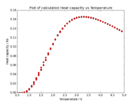
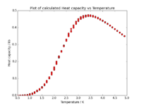
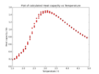
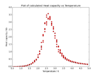
As we already have both the average energy and average squared energy, we can use the values and plot a graph of C [J/kB^2] vs T [J(kB] for each of our systems:

2x2	4x4	8x8	16x16	32x32

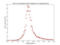
We can mention that the height of the peak grows approximately proportionally with $\sqrt{N}$.

One can mention, looking at the graphs above, that the Curie temperature is not the same, but is shifting towards lower values as the sample size is increased. It can be shown that this behaviour is governed by the following equation: $T_{C,L}=\frac{A}{\sqrt{N}}+T_{C,\mathrm{\infty }}$, where $T_{C,L}$ is the Curie temperature of a lattice with $N$ spins, $T_{C,\mathrm{\infty }}$ is the Curie temperature of an infinite lattice, and $A$ is an arbitrary constant.

Finding the Curie temperature of an infinite lattice

As mentioned above, the Curie temperature can be found as the temperature at which the maximum in system's heat capacity occurs. As the data around the phase transition regions are generally a bit noisy, it is more accurate to try fitting a polynomial to match our data, and determine the maximum of the polynomial:

data = np.loadtxt("NAME_OF_THE_FILE.dat") T = data[:,0] C = data[:,-1] # -1 just for an example, if the data only contain E, E2, and T, C can be calculated as (E2 - Esq)/(Tsq), where Esq = numpy.multiply(E, E) and #Tsq = numpy.multiply(T, T) Tmin = 2.0 #for example Tmax = 3.0 #for example selection = np.logical_and(T > Tmin, T < Tmax) #choose only those rows where both conditions are true peak_T_values = T[selection] peak_C_values = C[selection] #first we fit the polynomial to the data fit = np.polyfit(T, C, 100) # fit a third order polynomial #now we generate interpolated values of the fitted polynomial over the range of our function T_min = np.min(Tmin) T_max = np.max(Tmax) T_range = np.linspace(T_min, T_max, 1000) #generate 1000 evenly spaced points between T_min and T_max fitted_C_values = np.polyval(fit, T_range) # use the fit object to generate the corresponding values of C plt.plot(T_range, fitted_C_values, 'ro') plt.plot(T, C, 'ro') plt.show() Cmax = np.max(fitted_C_values) Tmax = T_range[fitted_C_values == Cmax] print Tmax

Fig. 7. Comparison of the dependence of heat capacity [$J/k_B^2$] on temperature [$J/k_B$] for a 32x32/C++ system (blue) and 32x32/Python system (red).

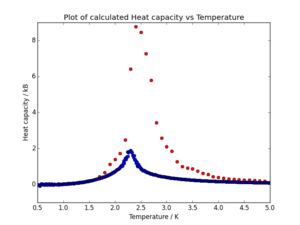
The polynomial always fits better at smaller ranges, so it is a good practise trying to fit the polynomial from Tmin to Tmax that are close to the peak.

For our calculations, the Curie temperature was found to be $2.59J/k_B$, not too far from the value given by Onsager,

$2.27J/k_B$.

C++

For comparison, much longer simulations has been run using C++, and the results of these simulations has been provided to us. Additionally, these results also contained a new, 64x64 system.

The data were extracted and plotted against our python data. An example can be seen in Fig. 7. Compared to our data, the values for Curie temperature were approximately about $0.3J/k_B$ smaller (the difference was higher, around $0.7J/k_B$, for smaller lattices, and smaller, around $0.2J/k_B$ for bigger ones).

The Curie temperature for an infinity lattice was found to be $2.285J/k_B$, this value is almost on par with the value of the theoretical calculations done by Onsager.

Magnetic susceptibility

Fig. 8. Graph showing the magnetic susceptibilities[$\mu /k_B$] vs temperature [$J/k_B$] for the 32x32/Python system (red) and the 32x32/C++ system (blue).

Magnetic susceptibility is a measure of the behaviour of a material under the magnetic field. It is negative for materials that are repelled by magnetic field and positive for materials attracted by magnetic field. It is dependent on the temperature of the system.

Using similar logic as above, it can be proven that:

$\chi =\beta (⟨M^2⟩-{⟨M⟩}^2)$

For 2D Ising lattice, the Onsager's solution for magnetic susceptibility is:

$\chi =\{\begin{array}{ll}0,& \text{if }T<T_c\\ decaying,& \text{otherwise}.\end{array}$

So we expect the susceptibility to be zero bellow the Curie temperature, abruptly rise to its maximum at the Curie temperature, and then slowly decay as the temperature goes higher.

Using a slightly changed code from above, magnetic susceptibility vs temperature were plotted for the 32x32/python and 32x32/C++ systems, and can be seen in Fig. 8. The actual values were rescaled so that the two curves can be compared, because the magnetic susceptibility of the C++ system was approximately $10^6$ times lower. We can see that the resolution of the C++ system is higher, probably because of the higher number of steps performed for the C++ system.

Magnetisation

Fig. 9. Dependence of magnetisation[$\mu /k_B$] on temperature [$J/k_B$] for the C++ systems. 2x2 system in red. 4x4 system in blue. 8x8 system in yellow. 16x16 in green. 32x32 system in cyan. 64x63 system in magenta.

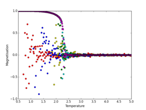
Using the more accurate C++ data, the behaviour of magnetisation (per spin) as a function of temperature was examined. Looking at Fig. 9, we can see that as the system size increases, the data fluctuate much less. For a 2x2 system, we can mention that the magnetisation fluctuates quite easily between 1 and -1 at temperatures bellow the Curie temperature, but as the system reaches the Curie temperature ( approx at $2.3J/k_B$) the data strongly converge to 0, as expected, as above the Curie temperature, entropy takes over and on average, the magnetisation cancels out. On the other hand, the 64x64 system (magenta in Fig. 9, plotted just by itself in Fig. 10), we can see that the magnetisation of the system fluctuates only around the Curie temperature. We can see an undershoot at that region. It is expected that this undershoot would slowly disappear as we would make the lattice bigger (Gibbs phenomenon), although this 'lability' is a natural behaviour of systems undergoing phase-changes, so we cannot neglect them completely. The magnetisation of the 64x64 system is approximately 1 at $T<<T_c$ and 0 at $T_{T}c$, with a quite abrupt change in magnetisation as we reach $T_c$ from left. This behaviour is expected, and in accordance with N. C. Young's solution at zero-field susceptibility :

Fig. 10. Dependence of magnetisation [$\mu /k_B$] on temperature [$J/k_B$] for the 64x64/C++ system.

$m(T)=\{\begin{array}{ll}(1-[sinh2\beta J{]}^{-4}{)}^{1/8},& \text{if }T<T_c\\ 0,& \text{if }T>T_c.\end{array}$

Energy

Fig. 11. Dependence of energy [$J$] on temperature [$J/k_B$] for the C++ systems. 2x2 system in red. 4x4 system in blue. 8x8 system in yellow. 16x16 in green. 32x32 system in cyan. 64x63 system in magenta.

As with magnetisation, the energy (per spin) of the C++ system as a function of temperature was examined. As mentioned before, the energy of the smaller systems (2x2 and 4x4) started at -2 J / spin and became gradually higher as the temperature of the system increased. The word 'gradually' is very important in this case, as for the larger system (16x16, 32x32 and 64x64), the change in energy was much steeper around the Curie temperature (Fig. 11). As opposed to the magnetisation studies, the size of the system had no observable effect on any random fluctuations. In fact, no fluctuations were observed whatsoever. This has mainly to do with the system reaching the lowest possible energy state for each increment in temperature. As the system is in a stable state, there is no 'driving' force for random fluctuations as seen for magnetisation.

Conclusion

In this experiment, various 2D Ising lattices were simulated using Python and their properties examined. The Curie temperature for each system was found, as well as the behaviour of average energy, average magnetisation, magnetic susceptibility and heat capacity of the system as functions of temperature. The results were then compared to the literature and to the C++ data provided to us. As a general trend, it was found that for the python data, the Curie temperature was slightly higher than for the C++ data and the Onsager's solution. This could probably be caused by not performing enough Monte Carlo steps for our energy/magnetisation calculation, and/or an incorrectly chosen range of Monte Carlo step for the average energy/average magnetisation. Although all calculations have been done 5 times for each system, it could be beneficial to run the calculations even more times to ensure any random fluctuations average out.

Considering the accuracy of our results, the C++ data files were more accurate than our Python data, behaving almost exactly as predicted by Onsager, Young, and others. Having to repeat this experiment, I would recommend:

1. Using a more powerful computer.
2. Perhaps using C++ to get more data more faster.
3. Using the biggest system possible.
4. If having not enough computational power, doing the computations for 16x16 system, as explained above.
5. Running the calculations even more times to ensure any fluctuations average out.
6. More deeply exploring the range of Monte Carlo steps needed to ensure 1) any fluctuations average out and 2) we don't include systems that are not in an equilibrium.

Literature sources