Rep:Mod:DOR1123

Introductory work and motivation

Molecular dynamics is a powerful tool that allows study of the movement of atoms and molecules in a system of interest. It is a so called "N-body" simulation which involves the study of a collection of particles that are acted upon by forces. The positions, velocities and forces of these particles can provide a wealth of information on how the system behaves as time elapses.

Alder and Wainwright, in 1957, used molecular dynamics to model perfectly elastic collisions between hard spheres. Their work, while simplistic in its execution, paved the way for further exciting developments in the field of molecular dynamics. The computational power available to a physical scientist has increased drastically in the last half century and as a consequence of this, so has the complexity of systems that may be examined. For example, modern applications of molecular dynamics include the modelling of large biomolecules (such as enzymes) and also the study of planetary orbits. Clearly, molecular dynamics is an invaluable asset to the modern researcher.

In this short report, the application of molecular dynamics to simulations of a simple fluid are discussed. While this may seem as far as possible from the elastic collisions of perfect spheres, this application came as a direct consequence of Alder and Wainwright's work. The theory of statistical thermodynamics along with the use of powerful software allows the determination of various thermodynamic properties of liquids. Molecular dynamics calculations can be compared to experimentally obtained quantities in order to strengthen the argument.

This report details an introductory experiment in molecular dynamics. Firstly, some simple input scripts are used in conjunction with a high performance computing software to measure thermodynamic data. The outputs of these introductory simulations are discussed in later sections. Then, some simulations are run whereby certain thermodynamic parameters are controlled, and equations of state are plotted. These equations of state are compared to predictions from the Ideal Gas Law. Subsequently, an input script is modified to allow determination of values of heat capacity for a system (using a different set of conditions; or ensemble). Radial distribution functions are discussed to provide an insight into the structural features of the systems under study. To conclude, mean square displacement and velocity autocorrelation functions are discussed to give some information on the dynamic properties of the system i.e. how the system behaves over time. The diffusion coefficient is discussed briefly; along with how it may be determined.

Theory and background

Discretisation and the velocity-Verlet algorithm

It is prudent to mention that the field of molecular dynamics leans to the more classical (rather than quantum mechanical) end of physics. While the distinction may become increasingly blurred as the appropriate theory becomes more complex, this level of work certainly relies heavily on Newtonian mechanics. In any case, exact solution of the Schrödinger equation for a system more complex than a hydrogen atom is impossible. As a result, these large systems of particles must be considered classically - this is a better approximation than one may think at first glance. Newton's laws of motion are fundamental to this area of physical chemistry. The theory behind molecular dynamics is rich and complex. It will not be discussed in detail here, unless absolutely vital to the task at hand.

As mentioned previously, Newtonian mechanics play a large part in the use of molecular dynamics. Newton's laws provide second order differential equations (involving acceleration, the second time derivative of position) for each and every atom in a particular system. The computation required increases rapidly - if there are 1000 atoms in a given system, 1000 solutions to these differential equations are required. Clearly, this cannot be done by hand. Note that it is most often the case that the system is to be studied over a period of time. In order to solve these differential equations using numerical integration, it is helpful to split the problem up into a series of discrete timesteps. This circumvents the need to treat the particle properties as continuous functions of time. The question remains - what type of integration is best to use?

An algorithm known as the velocity-Verlet algorithm provides a means of solving the necessary equations. It will not be described here, but, for all intents and purposes, it is a stepwise procedure which performs calculations based on initial conditions. As the properties that are to be calculated are discrete functions of time, this algorithm simply increases the timestep and outputs values. This procedure repeats until the desired time has elapsed - generating a collection of values for position and velocity at a collection of timesteps. A caveat of the velocity-Verlet algorithm is that initial positions of the atoms must be known, along with their initial velocities. Oftentimes, an iterative method may be applied for exactly this reason. Now, the results of the velocity-Verlet algorithm should be compared to those suggested by theory.

Below, a graph of position against time for a simple harmonic oscillator is shown. Both methods (analytical, and algorithmic) have been used to determine the position values; and they are plotted as separate data series.

Graph of position against time for a simple harmonic oscillator

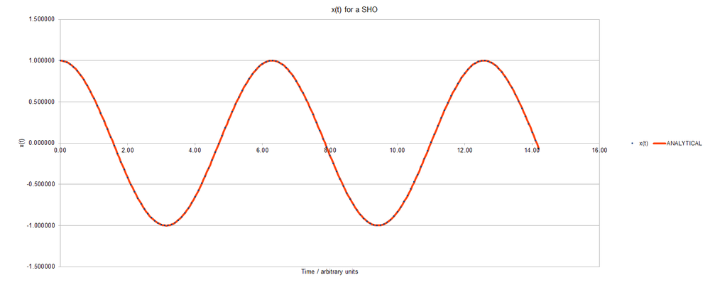
Looking at this graph, it may seem like the algorithm matches the analytical solution perfectly throughout the solution; but closer examination of the errors finds that this is not so. Shown below is a graph of the absolute error between analytical values and those determined by the algorithm.

Absolute error in velocity-Verlet calculations against time

Clearly, the errors become more significant at later times in the simulation. This phenomenon is better visualised with a plot of maximum error against time:

Maximum error against time

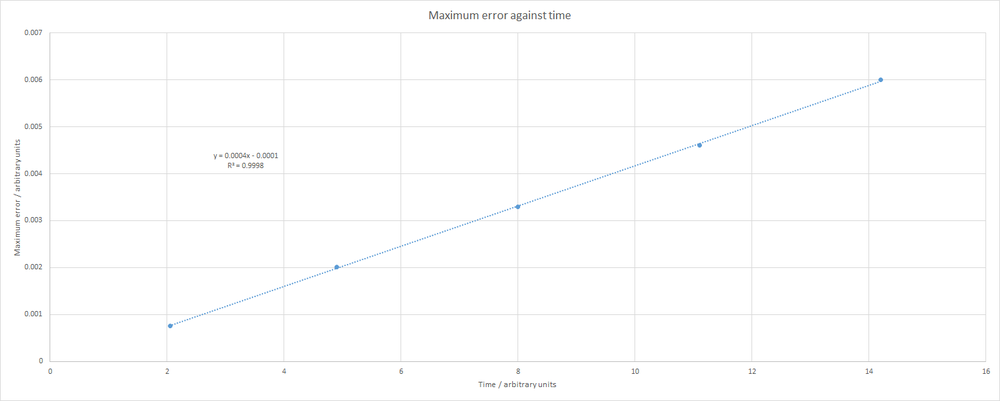
As seen, the maximum error increases linearly with time. The data are almost perfectly linear, with an R-squared equal to 0.9998. The equation that describes this line is shown on the plot. Note that all of the plots shown above correspond to a simulation with a timestep of 0.1. It is imperative that, when simulating a system of particles, the total energy remains effectively constant. An error of around 1 % should not cause too many problems. However, increasing the timestep can lead to difficulties. For example, below is a plot of total energy against time when using a timestep of 0.25.

Showing large discrepancy in total energy for a 0.25 timestep

This shows fluctuations in total energy of almost 2 %, which is unacceptable. Running the simulation at the original 0.1 timestep keeps the fluctuation to around 1 %. Any timesteps lower than 0.1 are also acceptable in that they maintain the total energy. However, having too low of a timestep means that many, many timesteps are required to simulate a small amount of overall time; therefore a balance must be struck.

Atomic Forces and Potential Energies

One step in the velocity-Verlet algorithm involves the calculation of the forces acting upon each atom. This calculation becomes complicated rapidly, as the force that each atom experiences depends on every other atom in the system. The equations necessary to determine these forces are quantum mechanical in nature and are not solved easily. Again, an approximation to classical physics is made. We can model the potential experienced between each pair of atoms using the Lennard-Jones potential. The force is then related to the potential by the following:

${\mathbf{F}}_i=-\frac{\mathrm{d}U}{\mathrm{d}{\mathbf{r}}_i}$

The Lennard-Jones potential for a single pair of atoms is as follows:

$\varphi \left(r\right)=4ϵ(\frac{{\sigma }^{12}}{r^{12}}-\frac{{\sigma }^6}{r^6})$

This models the potential curve shown below:

Lennard-Jones potential

Lennard-Jones potential

Manipulation of the Lennard-Jones potential can provide some useful information. For example; the separation at which the potential energy between the two particles is zero may be determined by simple algebraic manipulation. The Lennard-Jones potential can be set equal to zero:

$4ϵ(\frac{{\sigma }^{12}}{r^{12}}-\frac{{\sigma }^6}{r^6})=0$

Therefore;

$(\frac{{\sigma }^{12}}{r^{12}}-\frac{{\sigma }^6}{r^6})=0$

(if $ϵ$ is assumed to be non zero); and thus:

$\frac{{\sigma }^{12}}{r^{12}}=\frac{{\sigma }^6}{r^6}$

which can be rearranged to show that $r_0$ i.e. the separation at which the potential between particles is zero, is equal to $\sigma$. This matches up nicely with the graphical representation of a Lennard Jones potential that is shown above. The x-axis in this graph is $r/\sigma$. The x value of 1 corresponds to a potential of zero. This is expected from the result above.

It is then possible to use the relationship between force and potential to determine the force that acts at this separation. Differentiating the Lennard Jones expression and then substituting $\sigma$ for $r$ shows that the force at this separation is equal to $\frac{24ϵ}{\sigma }$.

Furthermore, another interesting point to examine on the potential is the equilibrium distance. This is the separation at which the potential is lowest i.e. the minimum. As force is a derivative of potential, the force will be zero at this point. Thus, setting the derivative of the LJ expression to zero and solving for $r$ shows that the equilibrium distance is $2^{\frac{1}{6}}\sigma$. This information may be used to calculate the well depth. The well depth is simply the pairwise potential at the equilibrium separation. Simple algebraic manipulation and substitution shows that the potential at $r_{eq}$ is $-ϵ$ therefore the well depth is $ϵ$. Again, these quantities can be easily seen on the potential curve.

Below, some integrals involving the Lennard-Jones potential are calculated:

$\underset{2\sigma }{\overset{\mathrm{\infty }}{\int }}\varphi \left(r\right)\mathrm{d}r=-0.025$

$\underset{2.5\sigma }{\overset{\mathrm{\infty }}{\int }}\varphi \left(r\right)\mathrm{d}r=-0.0082$

$\underset{3\sigma }{\overset{\mathrm{\infty }}{\int }}\varphi \left(r\right)\mathrm{d}r=-0.0033$

Note that for all of these integrals, $\sigma =ϵ=1$

Periodic Boundary Conditions and Reduced Units

Simulating realistic volumes of liquids would be extremely demanding, therefore most molecular dynamics simulations involve incredibly small volumes of liquid. To illustrate: consider than 1 mL of water contains approximately $3$x$10^{22}$ water molecules. In comparison, a simulation that models a system containing 10000 water molecules models a volume of around $3$x$10^{-19}$ mL. Although this is an incredibly large discrepancy, there is a computational tool that can provide a solution. Effectively, constraints are placed within the system whereby the walls of the simulation box are "continuous" i.e. if a particle reaches one of the boundaries, it will reappear at the opposite location to where it exited the box. For example, consider an atom in a simulation box that extends from (0,0,0) to (1,1,1). This atom is at (0.5,0.5,0.5) and moves through the vector (0.7,0.6,0.2). The atom ends up at (0.2,0.1,0.7). It will reach one of the boundaries, but continue through and reappear, as if it had never exited the simulation box.

Dimensional consistency is important in all mathematical and physical applications. A system of units (called reduced units) has been developed that is helpful when considering Lennard-Jones potentials. The "real" units are related to the reduced quantities by some constant. For example, in a system involving argon atoms, the LJ/cutoff command has an argument of 3.2 reduced units. In real units, this distance is 1.088 nm. The well depth, $ϵ$ is equal to $120k_B$ which can be written as $1.66E-21kJmo{l}^{-1}$. Finally, the reduced temperature, $120$ is equal to $180K$ in real units.

Equilibration

Examination of the input scripts

The simulations that were described in the introductory session provide outputs of thermodynamic data, depending on how the input file is written. The input file essentially defines a certain volume which is called the simulation box. The volume is define by a number of unit cells of a specified type. In this input file of the initial simulation; the first line reads:

lattice sc 0.8

This command specified a simple cubic lattice type with a number density of 0.8 and therefore creates a set of points that adhere to simple cubic geometry. The number density means that there are 0.8 unit cells per unit volume. The next part of the input script creates the simulation box that was mentioned before. The number of unit cells required in each of the Cartesian axes is specified. In this case, 10 x 10 x 10 is used. After the simulation box has been specified, it is necessary to perform the "create_atoms" command which will place an atom at each lattice point in the simlation box. Since there are 1000 unit cells in this particular simulation, the "create_atoms" command created 1000 atoms (as each simple cubic unit cell contains one lattice point). If a face centred cubic unit cell had been used, the "create_atoms" command would have created 4000 atoms - as a face centred cubic unit cell contains 4 lattice points; and there are 1000 unit cells.

Once the atoms have been created, their properties need to be specified. The input script contains:

mass 1 1.0 pair_style lj/cut 3.0 pair_coeff * * 1.0 1.0

The first line of this command tells LAMMPS that the atoms of type 1 will have a mass of 1.0 (in reduced units). The second line shown above has a twofold purpose. Firstly, it tells LAMMPS to use the Lennard-Jones potential (denoted "lj") and the formulae associated with this potential to calculate the potentials between neighbouring atoms. Secondly, the "cut" tells LAMMPS the cutoff distance for these pairwise interactions. In this case, any atoms greater than 3.0 distance units apart will not have a potential between them. Note that many different potentials are available (and there are even different types of Lennard-Jones potentials available). In summary, the "lj/cut 3.0" argument in the "pair_style" command means that LAMMPS will model the potential between atoms (less than 3 distance units apart) as a Lennard-Jones potential, but will not consider any Coulombic interactions. Ignoring Coulombic interactions is acceptable as the atoms we are considering are not charged species. The final command specifies which atoms are able to interact, and the coefficients for the force fields between the interacting atoms. The initial 2 asterisks mean that all atoms (i.e. atoms 1 to N) are able to interact with all other atoms 1 to N - of course an atom cannot interact with itself, however. Consider a pair of atoms, one labelled "i" and the other labelled "j". The values of i and j may be anything from 1 to N (remember that N is the total number of atoms in the system). The asterisks mean that any pair of atoms may interact, except when i is equal to j. The numerical arguments, "1.0 1.0" indicate the coefficients of the force fields used to model the pairwise potentials.

Therefore, 1000 atoms have been created so far, each with a known starting position (vertices of the simple cubic unit cell). The masses of the atoms and the forces between them have been set. Finally, the initial velocities need to be set. Since the initial positions and velocities of the atoms are being set, the velocity-Verlet algorithm may be used to determine the forces between the atoms in the system. Determining the initial positions required some thought, but providing initial velocities is considerable less involved. When a system of particles is at equilibrium, the velocities of the particles will follow a Maxwell Boltzmann distribution - the shape of which will be determined by the temperature of the system and the mass of the species. A command, described below, is used to tell LAMMPS how to determine the initial velocities. The input reads:

velocity all create 1.5 12345 dist gaussian rot yes mom yes

The command is known as the velocity command, and the "all" argument simply means that LAMMPS should assign velocities to all particles in the system. The word "create" is simply one of the styles that may be used to determine velocities. This particular style will generate a velocity for each atom using a random number generator, and will take 1.5 as the specified temperature. The "dist gaussian" portion of the line means that the velocities generated will follow a normal distribution, with a standard deviation that is scaled to follow the specified temperature. The "rot yes mom yes" argument will simply set the linear and angular momenta of all particles in a new ensemble to zero.

Now, the necessary properties of the system and of the atoms in the system have been specified. Next up, is to determine which thermodynamic properties can be monitored. The initial input file contains:

thermo_style custom time etotal temp press thermo 10

This tells LAMMPS to print the time, total energy, temperature and pressure in the log (output) file. It will do this every 10 timesteps.

When a number of different simulations need to be run it would be tedious to write a new input file for each and every one. This problem is overcome by the use of variables. Consider the lines below:

variable timestep equal 0.001 variable n_steps equal floor(100/${timestep}) timestep ${timestep} run ${n_steps}

The first line defines the variable called "timestep" to be equal to 0.001. The second line also defines a variable but is a little more complex. This defines a variable called "n_steps" to be equal to 100 divided by the value associated with the variable called "timestep". The meaning of the floor function is to avoid floating decimal points in the input file, and it essentially ensures that the variable "n_steps" is a pure integer number (with no associated decimal places). The third line specified that the timestep for this simulation should equal the value associated with the variable called "timestep". The final line tells LAMMPS to run the simulation for a number of timesteps equal to the variable called "n_steps". Note that throughout these lines, the element "${variable}" appears. This is in place to ensure that a new input file does not need to be written for each and every single simulation that is to be run. It is possible to simply redefine a variable; say "timestep" to a different value. This then will replace the value of timestep throughout all of the input script. The purpose of this is to make things simpler when running a large number of simulations when parameters must be varied often.

Discussion of outputs

All of this work that is done to: define a simulation box, create atoms, define their properties and tell LAMMPS what thermodynamic data to print in the log file would be much less useful if the system under consideration did not reach equilibrium (after all, the velocity command provides a distribution of velocities for a system assumed to reach equilibrium). Therefore, it is extremely important to be able to tell if a system reaches equilibrium. Equilibrium is characterised by a state in which the average values of thermodynamic properties become constant.

Shown below are some plots of thermodynamic parameters against time for the introductory simulation with a 0.001 timestep. Note that all units are in reduced form.

Plot of total energy against time for the 0.001 timestep simulation

Plot of temperature against time for the 0.001 timestep simulation

Plot of pressure against time for the 0.001 timestep simulation

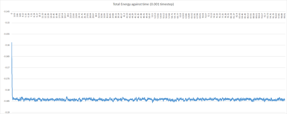
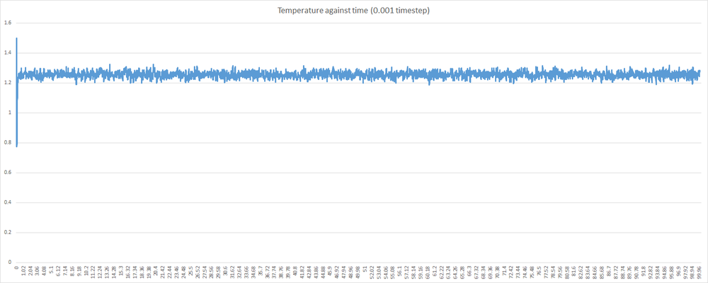
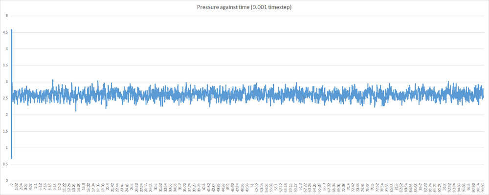
Examining the graphs above, it can be seen that the average values of total energy, pressure and temperature become constant after a small period of time. This indicates that the system used in the 0.001 timestep simulation does indeed reach equilibrium. This, however, is not the case for any timestep chosen. Some timesteps will prove problematic. Shown below is a plot of total energy against time containing a plot for each timestep. Examine the line for the 0.015 timestep - the average total energy is not constant. This is unacceptable, and 0.015 is a very poor choice of timestep. As a corollary, any timestep greater that 0.015 will be as bad a choice, if not worse.

Plots of total energy against time for each timestep

Examining the other 4 timesteps, one will see that the average total energy seems to depend on the nature of the timestep. This is not desirable, as the total energy should be an inherent property of the system, and obviously not depend on the level of discretisation. Thus, the largest timestep to give acceptable results will be the 0.0025 timestep. As mentioned before, a balance must be struck when choosing timestep - one must find the timesteps which minimise discrepancy in total energy; and then choose the largest of these. In this case, both the 0.001 and then 0.0025 timestep show least variation in the total energy; and 0.0025 is the largest.

Running simulations at specified conditions

NOTE: I ran these simulations with a 0.01 timestep, rather than a 0.0025. I made a mistake in determining acceptable timesteps, and the computer cluster was down on Thursday, so I was unable to redo the simulations at the correct timestep.

Theory and examination of input script

There are a number of different ensembles that may be used in molecular dynamics simulations. In simple terms, an ensemble determines a particular set of experimental conditions. There are the NVE (microcanonical), NVT (canonical) and NpT (isobaric-isothermal) ensembles. In this section, a simulation is run under the isobaric-isothermal ensemble. As the name suggests, this ensemble requires the user to specify a temperature and pressure in the input script. Throughout the simulation, these values are then held as close as possible to the specified values.

Pressures of 2.6 and 2.8 were chosen (again, in reduced units). The temperatures chosen were 1.6, 1.8, 2.0, 2.2, 2.4. The timestep chosen for these simulations was 0.01. These conditions provided 10 possible simulations - 5 temperatures at each pressure. The outputs of these simulations printed values of pressure, temperature and density. Also printed were the errors associated with each of these quantities.

The simulations that were run involved specifying temperature and pressure in the input script. The methods that LAMMPS uses to maintain isothermal-isobaric conditions should be discussed briefly. The equipartition theorem states that each degree of freedom in an equilibrated system has approximately $\frac{1}{2}{k}_{B}T$ of energy. Since there are N atoms in the systems being simulated, the total energy of the system (due to kinetic energy) may be written:

$E_{Kin}=\frac{3}{2}N{k}_{B}T$

LAMMPS uses this fact, and a calculation of instantaneous kinetic energy to determine the instantaneous temperature. The instantaneous temperature, $T$ will fluctuate, and often not be the same as the specified temperature, $\mathfrak{𝔗}$ and this needs to be accounted for. LAMMPS will perform a scaling of all velocities in the system to try and match the instantaneous temperature with the desired temperature. The velocities are scaled by a certain factor, $\gamma$. This factor will be less than one if the instantaneous temperature is greater than the desired temperature; and will be greater than one if the instantaneous temperature is too low.

Solving for $\gamma$ in the equations below:

$\frac{1}{2}\sum _i{m}_i{v}_i^2=\frac{3}{2}N{k}_{B}T$ $\frac{1}{2}\sum _i{m}_i{\left(\gamma v_i\right)}^2=\frac{3}{2}N{k}_B\mathfrak{𝔗}$

it is found that $\gamma =\sqrt{\frac{\mathfrak{𝔗}}{T}}$

Some of the input script for the isobaric-isothermal ensemble shall be examined below. Consider the line:

fix npt all npt temp ${T} ${T} ${tdamp} iso ${p} $ {p} ${pdamp}

The fix command tells LAMMPS to perform a certain type of integration. In this case it is a Nosé-Hoover algorithm (REF). This will cause the system to constantly perform an integration algorithm to correct both the pressure and the temperature. Two values of temperature and pressure are specified here, but they are, in fact, equal. These correspond to initial and final temperature values. In this case, the temperature and pressure must remain constant, so the values are the same. The "pdamp" and "tdamp" arguments indicate how often the temperature and pressure are to be calibrated. This command can often lead to problems, such as failure to reach equilibrium. These "damp" variables are chosen carefully to avoid these errors, and are often set as 100 timesteps. Therefore, in this simulation, calibrations will occur every time unit (as "timestep" variable is set equal to 0.01).

Now, the NpT ensemble has been set up and the isobar and isotherm should be maintained. Since the end goal of this section is to plot equations of state, average values of thermodynamic parameters need to be measured at certain intervals. Examine the lines:

fix aves all ave/time 100 1000 100000 v_dens v_temp v_press v_dens2 v_temp2 v_press2 run 100000

The values 100, 1000, and 100000 are of significance in these lines. The first number, 100, indicates that LAMMPS is to use thermodynamic parameters (temperature, pressure, density) as inputs every 100 timesteps. The value of 1000 means that LAMMPS should use the input values, from before, 1000 times for each average quantity that needs to be calculated. Finally, 100000 corresponds to the number of timesteps between calculations of average quantities (using the inputs and repeats from the previous numbers). In this case, the simulation runs only for 100000 timesteps, and therefore will result in only one set of average quantities being calculated for the entire simulation. In summary, this simulation will run for 1000 time units, and will calculate average quantities once throughout the simulation.

Equations of State

The values of density that were obtained using the input script described above were used to plot two graphs showing equations of state. Shown below is a plot of density against temperature at a pressure of 2.6. Included in the same axes is the plot of density against temperature that is predicted by the Ideal Gas Law.

Equation of state for pressure = 2.6

The simulated density shown above is lower than that predicted by the Ideal Gas Law. Below is another plot of an Equation of State; this time the pressure is equal to 2.8.

Equation of state for pressure = 2.8

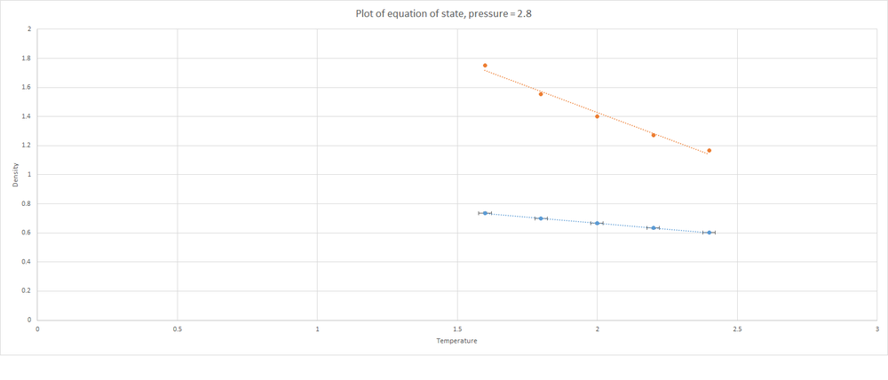
Again, see that the densities determined by the simulations are lower than those predicted by the Ideal Gas Law. This time the discrepancy between the values is even greater. The Ideal Gas Law states that atoms in a gas are not interacting unless they come into direct collision with each other. On the other hand, the Lennard Jones cutoff in the simulations is 3.0 units. These atoms will experience their neighbours much more than would be expected by the Ideal Gas Law. As a result, there is a larger region around atoms where it will be unlikely to find a neighbour; and so there will be fewer atoms per unit volume i.e. a lower density. This discrepancy increased with pressure. The atoms in the simulations will not experience much difference in how close they are to neighbours; wherea the Ideal Gas Law will predict that greater pressure (more atoms in a given volume) will certainly lead to an increase in density (and therefore an increase in the discrepancy between simulation and theory).

Calculating Heat Capacities

Thus far, input scripts have been provided. Manipulation of input scripts can open up a wide range of useful features in LAMMPS. Measurement of heat capacities using LAMMPS is discussed below.

Heat capacity, $C_v$ is equal to:

$N^2\frac{⟨E^2⟩-{⟨E⟩}^2}{k_B{T}^2}$

where, $N$ is the number of atoms in the system; $⟨E^2⟩$ is the average value of the energy squared; $⟨E{⟩}^2$ is the square of the average energy; $k_B$ is the Boltzmann constant and $T$ is the temperature.

In this section of the experiment, an input script was edited to provide a means of measuring the heat capacity of the system at varying densities. This involved changing some of the variables, and also defining new ones. An example of the input script may be found below:

Heat Capacity input script

Shown below is a plot of $C_v/V$ against temperature. Note that $V$ is the volume of the simulation cell.

Cv/V against Temperature for two densities

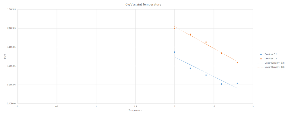
Note that for both plots, $C_v/V$ decreases as Temperature increases. Since the volume of the simulation box is constant, this is the trend that should be expected. Remember that heat capacity provides a measure of how much heat energy is required to raise the temperature of a system. Also, note that the $C_v/V$ values are larger for the more dense system. In the more dense system, more collisions between atoms will occur, and more energy will be lost during these collisions. Therefore, more energy must be placed into the system to increase the temperature that would be needed to increase the temperature of a less dense system.

Structural properties and the Radial Distribution Function (RDF)

If a atom in a system is set as a reference point, a circles of increasing radii may be drawn around this reference point. A function, known as the radial distribution function, can be used to examine the distances from this central reference atom that a neighbour is most likely to be found. Clearly, different densities and temperatures (i.e. different states of matter) will show a variety of radial distribution functions. In essence, it describes how number density of particles varies as a function of distance from a reference particle. The image below provides a pictorial representation of this phenomenon:

Schematic of the RDF

Schematic of the RDF

The radial distribution function may be determined using Visual Molecular Dynamics (VMD) software. As was mentioned in the introductory section, molecular dynamics simulations become more powerful when it is possible to compare their results to those obtained experimentally. The radial distribution function of a system may be determined by using neutron scattering, and this may then be compared with simulated values. See below for a plot showing the radial distribution functions for the solid, liquid and gas phases of the Lennard-Jones material.

RDF plots for solid, liquid and gas

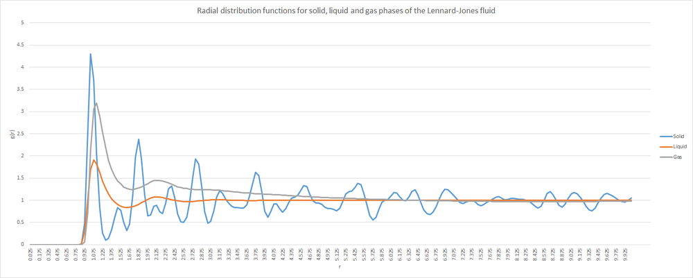
The most noticeable feature common to all states is that the RDF is zero for very small values of r. This is likely due to the atoms not being able to come any closer than a certain cutoff value of r. It represents the distance from the very centre of the reference atom to its outer shell i.e. the "diameter" of an atom. Clearly an atom cannot occupy a position inside another. The second feature that appears to be common to all states of matter is that the RDF will tend to 1 at large values of r. This is likely due to 1 becoming the average density of atoms at large distances. A greater volume is occupied as r increases, leading to a drop in the value of density; which will rapidly approach unity.

Next, consider the RDF for the solid phase. This shows peaks continuing to appear, even at large r. Any peaks in RDFs will correspond to a certain distance where neighbours are likely to be found. The fact that solids show peaks at large r implies a degree of long range order - something that is expected for solid materials. Furthermore, the peaks are sharp (moreso at lower r values) which would be characteristic of the extreme uniformity within a crystalline structure - remember that the face centred cubic lattice is the specified structure for the solid phase. The sharpness of the peaks is due to an atom in a crystal lattice having a negligible probability of appearing outside its lattice point. The regions where atoms in the solid may appear is very clearly defined. Since the lattice type is face centred cubic, the solid will adopt a close packed cubic structure, and the coordination number of each atom will be 12. The lattice spacing in this system may be determined using the simple formula: $L=2R\sqrt{2}$ where $L$ is the lattice spacing. In this case the lattice spacing is approximately equal to 3.04 reduced distance units.

Although peaks in the RDF are more characteristic of solids; clearly the liquid and gaseous phases also have peaks. This is due to there being a "shell" of neighbours around the reference atom. The lack of peaks at large r values for the liquid and gaseous phases is due to an increased level of disorder in the system. This is also the reason for the significant broadening of the peaks in these phases - the location of neighbours is less strictly defined, compared to solids.

Dynamical properties and the diffusion coefficient

Mean squared displacement

The mean squared displacement (MSD) is a tool used to evaluate the total distance travelled by a particular species over time. Note that the MSD has to be a squared quantity - this is due to the possibility of a "negative movement". Remember that displacement is a vector quantity, and if the negative displacement is allowed to alter the total distance travelled, then the value will not be representative of reality. Thus, the MSD is easily measured by recording the squares of each distance travelled. The Diffusion coefficient is related to the MSD by the following:

$D=\frac{1}{6}\frac{\partial ⟨r^2\left(t\right)⟩}{\partial t}$

Note that D is the diffusion coefficient, and is a constant that is used in defining the rate of diffusion.

Below is a plot of the MSD for a solid, liquid and gas. This system contains approximately 4000 atoms.

Mean squared displacement for solid, liquid and gas

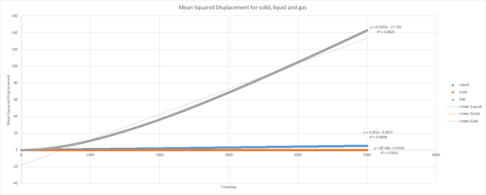
This trend in MSD as state of matter is varied is what one would expect. Remember that MSD is effectively a measure of how far each atoms travels on average during the simulation. The atoms in the solid rarely move at all during the simulation - the MSD value stays low even after many timesteps have elapsed. The liquid MSD increases to a larger value as more timesteps elapse. This is due to liquids having an increased disorder when compared to solids. The plot for the gas shows a very large MSD at longer time. The atoms in a gas are constantly moving, so the square of the distance travelled by gaseous atoms will obviously increase rapidly as time elapses.

This plot provides the values $D=0.00505m^2/s$, $D=0.00017m^2/s$ and $D=1E^{-8}{m}^2/s$ for gas, liquid and solid respectively.

The system described above was a quite small. Detailed below are the MSD for solid, liquid and gas phases in a 1 million atom simulation.

MSD for a 1 million atom simulation

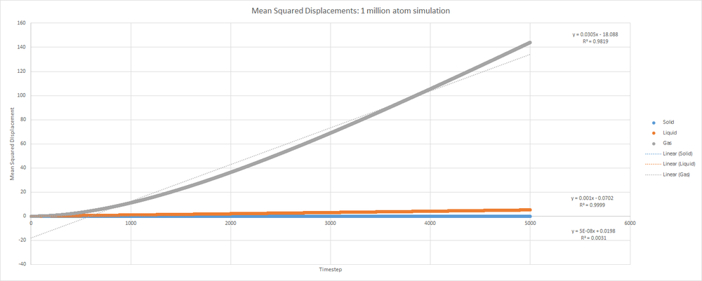
This plot provides the values $D=0.0051m^2/s$, $D=0.00016m^2/s$ and $D=8E^{-9}{m}^2/s$ for gas, liquid and solid respectively.

Velocity autocorrelation function

The diffusion coefficient may also be calculated using the velocity autocorrelation function (VACF). This function describes how correlated the velocity of an atom at time t is at a further time. It is expected that at large times, the correlation should equal zero as the velocity of a particle should not depend on its velocity much further back in time.

Shown below is the equation for the VACF of a one dimensional simple harmonic oscillator.

$C\left(\tau \right)=\frac{\underset{-\mathrm{\infty }}{\overset{\mathrm{\infty }}{\int }}v\left(t\right)v(t+\tau )\mathrm{d}t}{\underset{-\mathrm{\infty }}{\overset{\mathrm{\infty }}{\int }}{v}^2\left(t\right)\mathrm{d}t}$

Solving the numerator integral:

Remember that $x(t)=Acos(\omega t+\varphi )$ for a simple harmonic oscillator. Then, differentiating this expression to obtain an expression for the velocity of the simple harmonic oscillator at time t:

$v(t)=-\omega sin(\omega t+\varphi )$

Which corresponds to the function $v(t)$ in the 1D VACF integral above. Now, this function needs to be incorporated into the integral on the numerator of the VACF:

$\underset{-\mathrm{\infty }}{\overset{\mathrm{\infty }}{\int }}(-\omega sin(\omega t+\varphi ))(-\omega sin(\omega (t+\tau )+\varphi ))\mathrm{d}t$

Using the trigonometric substitution $sinAsinB=1/2(cos(A-B)-cos(A+B))$ and rearranging:

$\frac{{\omega }^2}{2}\underset{-\mathrm{\infty }}{\overset{\mathrm{\infty }}{\int }}(cos\left(\omega \tau \right)-cos(2\omega t+2\varphi +\omega \tau ))\mathrm{d}t$

Using the trigonometric identity $cos(A+B)=cosAcosB-sinAsinB$ and rearranging:

$\frac{{\omega }^2}{2}\underset{-\mathrm{\infty }}{\overset{\mathrm{\infty }}{\int }}(cos\left(\omega \tau \right)-cos\left(2\omega t\right)cos(2\varphi +\omega \tau )+sin\left(2\omega t\right)sin(2\varphi +\omega \tau ))\mathrm{d}t$

Note: I apologise, this last section was rushed. I did as much as I could before the deadline. Didn't manage my time very well.