Rep:Mod:Computational Liquids Will

Page for Liquid simulations experiment

Intro

Molecular dynamics aims to simulate systems under a simplified protocol to generate an understanding of real chemical systems. The complexity of chemical systems is great, with a wide variety of instantaneous forces constantly changing the parameters of the system. The aim of molecular dynamics is quite simply to find a way to model a system accurately, but in a way that allows computation. The ability to computationally simulate a system is of great benefit, and may allow the calculation of macroscopic properties assuming the system being simulated fulfills the ergodic hypothesis .

It is most common to approximate situations by solving Newtons equations for classical systems. Newtons second law can be utilized to generate an understanding of atomic interactions:

$$\begin{gathered} {\mathbf{F}}_i=m_i{\mathbf{a}}_i=m_i\frac{\mathrm{d}{\mathbf{v}}_i}{\mathrm{d}t}=m_i\frac{{\mathrm{d}}^2{\mathbf{x}}_i}{\mathrm{d}{t}^2} \\ (1) \end{gathered}$$

${\mathbf{F}}_i$ is the force acting on atom i. $m_i$ is the mass of atom i. ${\mathbf{a}}_i$ is the acceleration of atom i, the rate of change of its velocity. ${\mathbf{v}}_i$ is the velocity of atom i. ${\mathbf{x}}_i$ is the position of atom i.

The above equation allows the calculation of the position and velocities of the atom through knowing the force between them. However, there is an individual equation for each atom within our system, hence for an N atom system, there are N equations as above. This is almost impossible to quantify analytically, and hence molecular dynamic simulations use numerical methods, such as the verlet algorithm to simplify the problem. The Verlet algorithm operates very well, showing only minimal error, and preserves energy ( note energy must be conserved within a given system). However, the Verlet algorithm does not allow the calculation of Velocity and hence a modification known as the Velocity Verlet is often employed. The velocity verlet can generate output velocities, but requires an input initial velocity for the system. Luckily this can be well approximated by the Maxwell Boltzmann distribution, which gives the relationship between temperature and velocity.

Theory tasks

Velocity-Verlet algorithm

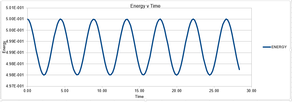
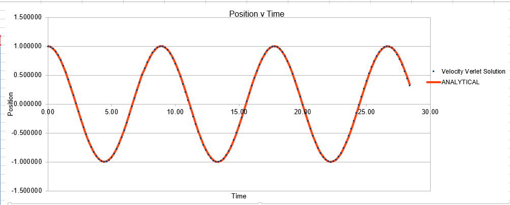
The Velocity Verlet solution was explored within an excel spreadsheet, comparing the solutions obtained to the classical model. The data calculated included the position of the atom( calculated using a classical harmonic oscillator such: $x\left(t\right)=A\cos (\omega t+\varphi )$) The energy of the data set was also calculated, whereby the energy of the velocity verlet was calculated via: $E=\frac{1}{2}m{v}^2+\frac{1}{2}k{x}^2$

Where m=mass v= velocity k=force constant x= position

First Set Parameters for this data: Timestep =0.1 Mass=1.0 k=1 X(0)=1.00 V(0)=1.00 Phi=0.00 A=1 Omega=1.00 ‎

Second Set

Parameters for this data: Timestep =0.2 Mass=1.0 k=1 X(0)=1.00 V(0)=1.00 Phi=0.00 A=1 Omega=1.00

‎

Third Set

Parameters for this data: Timestep =0.5 Mass=1.0 k=1 X(0)=1.00 V(0)=1.00 Phi=0.00 A=1 Omega=1.00

Fourth Set

Parameters for this data: Timestep =0.05 Mass=1.0 k=1 X(0)=1.00 V(0)=1.00 Phi=0.00 A=1 Omega=1.00

‎

‎

Examining the Timestep

In order to establish an accurate system it is optimal for the total energy of the system to not change by 1% ( remembering that in a true system the total energy should be remaining completely constant). The graphs above demonstrate that the limit for this behavior is a time step of 0.2, with the graph displayed again below for convenience. It can be clearly evidenced that when an excessive timestep was used ( 0.5) the error in the system was considerably larger than 1%. Finally it should also be noted that although 0.1 timestep gives a lower error, it would likely be more computationally expensive to run. From the above graphs it is recommended that a time step of 0.2 is utilized

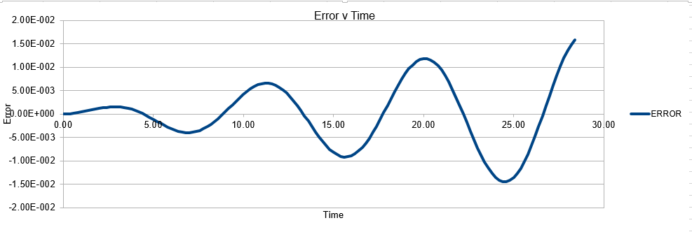
Prompt questions: Why do you think it is important to monitor the total energy of a physical system when modelling its behaviour numerically? Why do you think the error in the position changes with time in the way that it does?

As mentioned above, it is important to measure the total energy of a physical system as it should be adhering to the conservation of energy law, and thus maintaining a constant value. Monitoring the energy of the system allows one to make a induction as to the likely accuracy of the system. Of course it may not always be the software that is insufficent, it may be the input code is incorrectly written, and thus is leading to changes in energy

The error obtained is a result of the velocity verlet and the manner in which it is calculated. Its source is based on the position of the atom, whereby there is a constant cumulative error as the system is being run accompanied with an error in the new position of an atom. Hence this is why the error begins very small near the beginning of the simulation, and grows as the simulation proceeds. This is because the velocity verlet is based on a taylor expansion, which loses accuracy at large (t). Due to the error being associated with position, any input that acts to increase the velocity, will increase the error.

Examining the Mass

The mass of the system was varied due to the simple relationship of the frequency of vibration and the mass such

$\omega =\sqrt{\frac{k}{\mu }}$

Thus we expect that increasing the mass will lead to a reduced value of frequency. The expected result is evidenced below:

Mass 0.5

‎

Mass 2.0

 ‎ 

‎

‎

Calculations from Theory Subsection

Find the separation, $r_0$, at which the potential energy is zero $\varphi \left(r\right)=4ϵ(\frac{{\sigma }^{12}}{r^{12}}-\frac{{\sigma }^6}{r^6})$

When $\varphi (r)=0$, it follows that:

$0=4ϵ(\frac{{\sigma }^{12}}{r^{12}}-\frac{{\sigma }^6}{r^6})$, therefore:

$0=(\frac{{\sigma }^{12}}{r^{12}}-\frac{{\sigma }^6}{r^6})$

$(\frac{{\sigma }^{12}}{r^{12}})=(\frac{{\sigma }^6}{r^6})$

and therefore for $\varphi (r)=0$, $r=\sigma$

Calculate the force at this separation, for the case $\varphi (r)=0$

Where $\varphi (r)=0$, $r=\sigma$

In the Lennard Jones model , $Force=F=\frac{-d\varphi (r)}{dr}$

$\frac{-d\varphi (r)}{dr}=-4ϵ(\frac{-12{\sigma }^{12}}{r^{13}}+\frac{6{\sigma }^6}{r^7})$

Invoking where $\varphi (r)=0$, $r=\sigma$

allows the simplification: $-4ϵ(\frac{-12{\sigma }^{12}}{r^{13}}+\frac{6{\sigma }^6}{r^7})=-4ϵ(\frac{-12}{\sigma }+\frac{6}{\sigma })$

Therfore $F=\frac{24ϵ}{\sigma }$

Calculate the equilibrium separation

For this separation $r=\sigma$ is no longer valid.

$F=\frac{-d\varphi (r)}{dr}=-4ϵ(\frac{-12{\sigma }^{12}}{r^{13}}+\frac{6{\sigma }^6}{r^7})=(\frac{48ϵ{\sigma }^{12}}{r^{13}}-\frac{24ϵ{\sigma }^6}{r^7})$

At equilibrium distance, $F=O$

$0=(\frac{48ϵ{\sigma }^{12}}{r^{13}}-\frac{24ϵ{\sigma }^6}{r^7})$

$(\frac{48ϵ{\sigma }^{12}}{r^{13}}=\frac{24ϵ{\sigma }^6}{r^7})$

$(\frac{2{\sigma }^6}{r^{13}}=\frac{1}{r^7})$

$2{\sigma }^6=r^6$

$r=\sigma \sqrt[6]{2}$

Working out well depth

The well depth can simply be calculated with:

$\varphi \left(r\right)=4ϵ(\frac{{\sigma }^{12}}{r^{12}}-\frac{{\sigma }^6}{r^6})$

$r=\sigma \sqrt[6]{2}$

Substitution and simplification obtains: $4ϵ(\frac{1}{4}-\frac{1}{2})$

And thus the well depth $=-ϵ$

Evaluate the integral $\underset{2\sigma }{\overset{\mathrm{\infty }}{\int }}\varphi \left(r\right)\mathrm{d}r$

when $\sigma =ϵ=1.0$

$\varphi \left(r\right)=4ϵ(\frac{{\sigma }^{12}}{r^{12}}-\frac{{\sigma }^6}{r^6})$

Therefore: $\underset{2\sigma }{\overset{\mathrm{\infty }}{\int }}\varphi \left(r\right)\mathrm{d}r=\underset{2\sigma }{\overset{\mathrm{\infty }}{\int }}4ϵ(\frac{{\sigma }^{12}}{r^{12}}-\frac{{\sigma }^6}{r^6})$

$=4\underset{2\sigma }{\overset{\mathrm{\infty }}{\int }}(\frac{1^{12}}{r^{12}}-\frac{1^6}{r^6})$

$=4[\frac{-r^{-11}}{11}+\frac{r^{-5}}{5}]{|}_2^{\mathrm{\infty }}$ Please note the limits here are supposed to be between $2\sigma$ and $\mathrm{\infty }$

=$4(0-((\frac{-1}{11}\times \frac{1}{2^{11}})+(\frac{1}{5}\times \frac{1}{2^5}))$ $=-2.48\times 10^{-2}$

Evaluate the integral $\underset{2.5\sigma }{\overset{\mathrm{\infty }}{\int }}\varphi \left(r\right)\mathrm{d}r$

when $\sigma =ϵ=1.0$

The working is exactly analogous to above until the limits are applied:

=$4(0-((\frac{-1}{11}\times \frac{1}{2.5^{11}})+(\frac{1}{5}\times \frac{1}{2.5^5}))$

$=-8.18\times 10^{-3}$

Evaluate the integral $\underset{3\sigma }{\overset{\mathrm{\infty }}{\int }}\varphi \left(r\right)\mathrm{d}r$

when $\sigma =ϵ=1.0$

The working is exactly analogous to above until the limits are applied:

=$4(0-((\frac{-1}{11}\times \frac{1}{3^{11}})+(\frac{1}{5}\times \frac{1}{3^5}))$

$=-3.29\times 10^{-3}$

Volume and number of Water Molecules

TASK: Estimate the number of water molecules in 1ml of water under standard conditions. Estimate the volume of 10000 water molecules under standard conditions.

Cubic Simulation Atomic position TASK: Consider an atom at position $(0.5,0.5,0.5)$ in a cubic simulation box which runs from $(0,0,0)$ to $(1,1,1)$. In a single timestep, it moves along the vector $(0.7,0.6,0.2)$. At what point does it end up, after the periodic boundary conditions have been applied?.

After a single timestep, the atom will be located at (0.2,0.1,0.7)

Lennard-Jones parameters and reduced units

LJ cutoff = $3.2\times 0.34=1.088nm$

Well depth ( previously defined)$=-ϵ$

$=\frac{120\times k_b\times N_a}{1000}$

$=-0.997\frac{kJ}{mol}$

Reduced T$=1.5(120)=180$

Equilibration

TASK: Why do you think giving atoms random starting coordinates causes problems in simulations? Hint: what happens if two atoms happen to be generated close together?

The inherent problem with giving random starting coordinates should be somewhat obvious- although chemical systems may appear highly fluxional and at times atomic behaviour may seem random, there are many underlying attractive and repulsive forces that account for this motion. The main issue with applying a random configurations is the underlying assumption that goes with this, that all configurations of a system share the same probability of occurrence, and hence the systems state can be described by a random arrangement. Analyzing this interpretation leads to a huge number of theoretical flaws. Taking water as an example, in either the solid or liquid phase the arrangement of the molecules is such to allow hydrogen bonding, there is an inherent system preference for the molecules to align as such to maximise these favourable hydrogen bonding interactions. The intermolecular distances in water can thus be considered a resultant of these interactions. Computational simulation could begin to account for this through initializing the simulation with the molecules orientated in such a way as to facilitate hydrogen bonding, and this is suggestive that a random starting position is not optimal.

To further generalise the problem, imparting randomness will not account for the highly unfavourable interactions that take place at low interatomic distance, as predicted through the Lennard Jones potential. The problem with initializing a calculation with multiple atoms at very close inter nuclear distance would lead to complications within the simulation, either leading to an incorrect simulation, or enhanced computational time before a correct solution is obtained.

TASK: Satisfy yourself that this lattice spacing corresponds to a number density of lattice points of 0.8. Consider instead a face-centred cubic lattice with a lattice point number density of 1.2. What is the side length of the cubic unit cell?

TASK: Consider again the face-centered cubic lattice from the previous task. How many atoms would be created by the create_atoms command if you had defined that lattice instead?

As this lattice has 4 atoms per unit cell, compared to the 1 atom per unit cell of the standard cubic lattice, replacing the cubic lattice with the face centered cubic generates 4 times as many atoms as previously. Therefore, the number of atoms generated in this case is 4000

Setting the properties of the atoms

TASK: Using the LAMMPS manual, find the purpose of the following commands in the input script:

mass 1 1.0
pair_style lj/cut 3.0
pair_coeff * * 1.0 1.0

Mass This command is in the general of mass I value, where I= the atom type and value represents the value of the mass of the respective atom. In the instance listed above, mass 1 1.0 can be interpreted as atom type 1 having a mass of 1.0.

The generality of this command can be increased utilising other inputs replacing the atom type section of the input, such:

mass 1 1.0: Exactly as above, atom type 1 has mass of 1.0

mass * 1.0: Asterisk notation with no numerical value is interpreted as all of the atom types ( from 1 to N, where N is the number of atom types). In this instance this input line would mean all atom types from 1 to N have mass 1

mass 10* 1.0: A leading asterk means all types from 1 to n ( inclusive). In this case this input line would mean atoms 1 to 10 have mass 1.0, but gives no input as to the mass of any atoms from n to N.

mass*10 1.0: A trailing asterisk is the contrary to the above, and represents a command for all atoms n to N. In this instance this input line would give all atoms from 10 to N a mass of 10, but gives no input as to the mass of any atom type below 10

mass 2*10 1.0: An asterisk between two values only gives restrictions on these values. Such, this input line would generate all atoms between 2 and 10 ( inclusive) with mass 1.0.

pair_style lj/cut 3.0

This command computes interactions between pairs, and in this instance is calculating interactions using the Lennard Jones Potential $\varphi \left(r\right)=4ϵ(\frac{{\sigma }^{12}}{r^{12}}-\frac{{\sigma }^6}{r^6})$. The 3.0 represents the cutoff distance for any interaction, above this distance the program will not compute any interaction

It should be noted that the pairwise interaction calculated here is perhaps the most simple variable of this command. Possible extensions including requiring LAMPS to calculate Coulombic terms.

pair_coeff * * 1.0 1.0

This command takes the general form of pair_coeff I J args, where I must be less than J or else the command line will be ignored. The command specifies the pairwise force field coefficients for one or more pairs of atom type.

TASK: Given that we are specifying ${\mathbf{x}}_i\left(0\right)$ and ${\mathbf{v}}_i\left(0\right)$, which integration algorithm are we going to use?

We will be using the verlet velocity algorithm as we are specifying the starting positions and velocities of the atoms.

Examining the Script

TASK: Look at the lines below.

### SPECIFY TIMESTEP ###
variable timestep equal 0.001
variable n_steps equal floor(100/${timestep})
variable n_steps equal floor(100/0.001)
timestep ${timestep}
timestep 0.001

### RUN SIMULATION ###
run ${n_steps}
run 100000

The second line (starting "variable timestep...") tells LAMMPS that if it encounters the text ${timestep} on a subsequent line, it should replace it by the value given. In this case, the value ${timestep} is always replaced by 0.001. In light of this, what do you think the purpose of these lines is? Why not just write:

timestep 0.001
run 100000

Writing the code in the longer form is necessary to aid the ease of varying the timestep. In the modified shortened version, the total time of the simulation is the timestep (0.001) multiplied by the number of runs (100000) of this timestep. If we doubled the timestep to 0.002 we would then be doubling the overall time of the simulation. For comparable results we need to simulation for the same length of time within simulations, and thus if we cahnged the timestep, we would need to alter the run line as well to account for this change.

This simplified example perhaps does not adequately stress the benefit of the elongated script. By using the elongated script we can vary the timestep, and without further modification the script will always simulate the same total time. Despite the appearance of the elongated script, it actually results in easier computation.

Output Files

Make plots of the energy, temperature, and pressure, against time for the 0.001 timestep experiment (attach a picture to your report)

Does the simulation reach equilibrium?

From examining these graphs it appears as though the system may reach equilibrium, but at this scale it is particularly difficult to tell. In order to examine if equilibrium is achieved the horizontal scale needs to be shortened, and the value around which the system oscillates found. In order for equilibrium to be established we will be looking for oscillation around a very small range.

How long does it take

The graphs below represent a enlarged scale of the previous graphs in order to aid visualisation of when equilibrium is obtained

It can be seen that equilibrium is consistently achieved when t= 0.35- 0.40

Make a single plot which shows the energy versus time for all of the timesteps

The below graph shows the total energy against timestep for all five graphs. This graph allows the conclusion that any time step is valid, except the highest value of timestep ( 0.15). The validity of this conclusion will be addressed further below with an enlarged scale

Of the five timesteps that you used, which is the largest to give acceptable results? Which one of the five is a particularly bad choice? Why?

As can be seen from the above diagram, the time steps of the highest accuracy are 0.001 and 0.0025. It was established above that the 0.15 time step was particularly bad, but it also appears the 0.01 and 0.015 are not particularly good at representing the system. With the equilibrium value having a reasonable degree of oscillation. In monitoring this system it would actually make sense to use the slightly higher timestep 0.0025 than 0.001. This timestep gives almost analogous results to the lower timestep, and will be less computationally expensive to run. In an ideal situation we would chose to model all systems with the lowest possible timestep, in order to best produce reality. Computational expense however means that more often than not we are actually looking for the highest timestep that still gives accurate results, in this instance probably t=0.0025

Running Simulations Under Specific Conditions

Choose 5 temperatures (above the critical temperature $T^{*}=1.5$), and two pressures to give ten phase points ( five temperatures at each pressure. You should be able to use the results of the previous section to choose a timestep

From the preceding graphs it can be determined that the equilibrium pressure oscillates around a value of approximately 2.5. The two pressures chosen to model similar systems were thus 2.4 and 2.6. The temperatures chosen were 1.6, 2.5,5 and 10, with all of these values being above the critical temperature. The critical temperature represents the temperature at which the molecules possess so much kinetic motion it is impossible to liquify them. Thus by choosing temperatures only above the critical temperature, we can be sure that our system is running in an entirely gaseous phase.

Solve the following equations to determine $\gamma$

Equation 1:

$\frac{1}{2}\sum _i{m}_i{v}_i^2=\frac{3}{2}N{k}_{B}T$

Equation 2:

$\frac{1}{2}\sum _i{m}_i{\left(\gamma v_i\right)}^2=\frac{3}{2}N{k}_B\mathfrak{𝔗}$

Division of Equation 2 by Equation 1 gives:

${\gamma }^2=\frac{\mathfrak{𝔗}}{T}$

Therefore:

$\gamma =\sqrt{\frac{\mathfrak{𝔗}}{T}}$

Use the LAAMPS Manual to find out the importance of the three numbers 100 1000 100000 in the exert of the script below. How often will values of the temperature, etc., be sampled for the average? How many measurements contribute to the average? Looking to the following line, how much time will you simulate?

### MEASURE SYSTEM STATE ###
thermo_style custom step etotal temp press density
variable dens equal density
variable dens2 equal density*density
variable temp equal temp
variable temp2 equal temp*temp
variable press equal press
variable press2 equal press*press
fix aves all ave/time 100 1000 100000 v_dens v_temp v_press v_dens2 v_temp2 v_press2
run 100000

The fix aves all ave/time 100 1000 100000 v_dens v_temp_v_press v_dens2 v_temp2 v_press 2 line is essentially telling LAAMPS to calculate the averages of the variables listed at the end of this line ( denisty, temperature, pressure, density 2, temperature 2 and pressure 2). In order for this line to function correctly every variable that is being averaged must be previously defined, such adding in v_etotal in to the averaging line would not function correctly, as etotal is not a defined variable. In order to make this line function the line : 'variable etotal equal etotal' would have to be defined. Further only variables stated in the thermo_style line can be defined. Although the thermo style line can be modified to include further system properties.

The numbers on the fix aves line refer to: take a sample every x steps |take x samples total| continue for x timesteps.

Of course of the three numbers present, only 2 are variables, with the third being a consequence of the other 2. In the instance listed above, we are taking a sample every hundred steps, taking 1000 samples total, and thus are continuing for ( 100*1000) timesteps.

Total time is simply # of timesteps * timestep. For this reason the amount of time the system is simulating can be varied without any changes to the displayed script above, and rather can be altered by modifying the value of the timestep.

Use software of your choice to plot the density as a function of temperature for both of the pressures that you simulated. Your graph(s) should include error bars in both the x and y directions. You should also include a line corresponding to the density predicted by the ideal gas law at that pressure. Is your simulated density lower or higher? Justify this. Does the discrepancy increase or decrease with pressure?

The main two assumptions of the ideal gas law state that the gas molecules themselves have no volume, and that these molecules have no attractive forces between one another. These assumptions are valid at very low pressures, where the volume of gas atoms is a very low proportion of the total volume of the container and the distances between atoms are so large that there is very little potential energy interactions.

However at higher pressures, the molecules can interact with one another and the ideal gas law overestimates density because it underestimates repulsive interactions between atoms. This means the ideal gas law has too many particles in a given volume, because it is not taking account of the repulsive Lennard Jones interactions that are present in the system at small distances. It should also be noted that for a system containing a very large number of atoms, the volume of the atoms themselves begin to make a significant contribution to volume, this is another reason why the ideal gas law predicts a higher density.

The effects are magnified at higher pressures, whereby interatomic interaction is more likely. The discrepancy is however lowered by temperature, the kinetic energy provided by increasing T is enough to overcome the attractive interactions. As we move to higher and higher T, we can expect our interactions to become more ideal. Thus if we want to model an ideal gas within a simulation we should model at very high T and low P.

Calculating heat capacities using statistical physics

A script was written ( example script here) in order to allow the calculation of the heat capacity of the system, following the equation:

$C_V=\frac{\partial E}{\partial T}=\frac{\mathrm{V}\mathrm{a}\mathrm{r}\left[E\right]}{k_B{T}^2}=N^2\frac{⟨E^2⟩-{⟨E⟩}^2}{k_B{T}^2}$

where the script creates a system composed of 3375 atoms, with lattice length 16.1583

The ensemble used for this calculation is the canonical ensemble, which differs from the isothermal/ isobaric ensemble in that work energy is no longer able to exchange with the surroundings. In the canonical ensemble the only parameter for exchange is q. It is important to note that although working in the canonical ensemble allows for easier computation, it isnt necessarily the most optimal way to model a chemical system ( most chemical reactions involve gas release, and thus involve a variable volume).

The obtained results are displayed below:

For Lattice Density of 0.2

Temperature	Heat Capacity
2.0	0.24289772
2.2	0.183825488
2.4	0.156341617
2.6	0.115348018
2.8	0.077391013

For Lattice Density of 0.8

Temperature	Heat Capacity
2.0	0.099581695
2.2	0.079311065
2.4	0.064950515
2.6	0.057482461
2.8	0.052541401

Graphical Representation of Heat Capacity against Temperature

What about the heat capacity at constant volume?

The script produces a cube of side 16.1583. Therefore the volume of the cube is 4218.78. Division of the heat capacty values above by the volume of the cube allows the obtainment of the heat capacity at constant volume

Is the trend what you would expect?

Firstly we need to consider what exactly the heat capacity represents. The heat capacity denotes the energy required to raise the systems temperature. A simple prediction therefore would be that higher density would lead to an increased heat capacity. Because we have the constraint of having a constant number of atoms, we know that the system with a higher density must achieve this by having a smaller volume. A smaller volume, but with the same number of atoms must lead to a higher heat capacity, and this is evidenced in the graphs above.

To take a more statistical mechanics view: The heat capacity is actually a measure of variance within the system, whereby the heat capacity gives the variance of internal energy, and reflects the ease of exciting the system to a higher energy state. At very high T however, all the molecules can access all the energy levels, and the system cannot absorb any more energy, thus the heat capacity begins to tend towards zero as T gets very high.

Structural properties and the radial distribution function

In this section, the calculation of the radial distribution function will be discussed. In the simplest terms, the radial distribution function represents the probability of finding a particle a distance r away from a reference particle. The key word within this statement is 'probability', whereby this term necessitates a reference system which is usually an ideal gas. The radial distribution function is a critical quantity to be able to calculate. Firstly it gives valuable information as to the density of a system, and can also be used to determine other thermodynamic quantities. Secondly the radial distribution function can be determined via experimental means, this allows comparison between a theoretical system and a real one, and allows one to determine the effectiveness and accuracy of a given simulation.

What do we expect to find?

We are going to model a solid, liquid and gas with the simulation, and analyse the radial distribution output. The gas output should be expected to be simplest, remembering our model is a ideal gas, the simulation of the gas shouldn't be all that different. The graph should display a single isolated peak that approaches 1 if it our model is similar to that of a free gas.

For the solid we expect the radial distribution function to exceed 1 in a variety of places along the graph. A solid is of course more dense than an ideal gas, and thus the radial distribution function will show a higher probability of finding a neighbour at a wide range of distances within a solid. It can be expected that the solid peaks within the radial distribution will be sharper than for the liquid or gas. The solids rigid lattice structure allows for little atomic movement meaning interactions occur only at very precise distances in accordance with the lattice structure. This is not true for liquids or gases, where we expect the greater degree of freedom within the systems to give broader peaks due to increased atomic motion. Unfortunately there was insufficient time, but it was postulated that increasing the temperature of these simulations may lead to a broadening of the peaks due to the enhanced atomic motion.

We can expect the liquid phase to have appearance inbetween that of the solid and the gas, with no particular long range order.

The system parameters used are defined below, followed by graphical representations Solid: X Density X Temperature Liquid: X Density X Temperature Gas: X Density X Temperature

Solid

Liquid

Gas

Plot the RDFs for the three systems on the same axes, and attach a copy to your report

What does the above tell us about the lattice system in each phase?

The systems are very similar to what we predicted, and display information as to the ordering within the structures. Perhaps of note however is the vapour, which is indicative that our model system is not representative of an ideal gas. An ideal gas ( the reference system for the model) would be expected to produce a straight horizontal line at a radial distribution equal to 1 for all r values. The presence however of a distinct peak suggests our model gas does indeed have interactions, and thus has a optimal or most favourable distance for atoms to be apart. Note however that at long r distances, our system begins to adopt a configuration identical to that of an ideal gas. As expected, the solid gives the sharpest peaks due to the restriction of atomic motion as mention previously. Theoretically for a perfect crystal a delta function would be expected, however inherent system defects and a slight degree of atomic motion acts to broaden this delta function in to the observed peaks. The defects are entropically driven, and have the main consequence of effecting system order. Schotky and Frenkel defects are intrinsic defects, with a Schotky defect causing a decrease in density due to a missing atom, and a Frenkel defect having no effect on density, representing a movement of an ion to fill a hole. As the radius increases, the probability of encountering defects increases, and thus at longer radial distances, the peaks begin to broaden out more significantly due to a loss of order. Thankfully, even at long r distances the solid is showing no sign of maintaining a constant radial distribution, it maintains a degree of order far higher than that of the reference system even at these high r values. The liquid phase also displays a degree of order, but at long r distances it can be noted that the system does begin to model identical characteristics to the ideal gas.

In the solid case, illustrate which lattice sites the first three peaks correspond to.

The first three peaks should correspond to the nearest three atoms For an FCC lattice:

From the above referenced diagram, the three closet neighbors are labelled A, B and C. These correspond to the first three peaks, where A is the first peak, B the second and C the third.

What is the lattice spacing?

In the reference diagram above, the distance between the reference atom, and atom B represents the lattice spacing. This distance in turn correlates to the second peak in the radial distribution (whereby the first peak represents the closest atom A). By examining this value, we obtain a value of 1.55 for the lattice spacing parameter.

What is the coordination number for each of the first three peaks?

The coordination number is obtained by examining the peaks and the running integral in turn. For the closest neighbour, the coordination is found firstly by examining the value at which the first peak begins to collapse, and then comparing this value of r the running integral at the same value of r. For the case of the first peak, it begins to diminish just above 1, and this corresponds to the running integral of 12 ( with rounding for non whole atoms). Repeating the same process for the second and third peaks gives running integrals of 18 and 43 respectively. However these values must have the areas of preceding peaks subtracted from them. Hence the second nearest neighbour has co-ordination number (18-12)=6. The third nearest neighbour has coordination number 43-18=25. Intuitively this final value seems a little out, expanding the crystal equally in all dimensions should return an even co-ordination number.

The overall co:ordination numbers for the first three peaks are 12:6:25, where an error is suspected in the final value

Dynamical properties and the diffusion coefficient

What does the MSD represent, and what do we expect it to show?

The MSD can be intuitively thought of as the distance explored by any one atom. With this idea in mind, we can begin to envisage what the system might look like. For a liquid we simply expect a linear increase with time. An analogy of a movement in a liquid would be trying to make your way through a very crowded area. Although your movement technically holds very little restrictions, you will find it hard to move any significant distance quickly, but, given enough time you can explore the whole area. Motion in a liquid is very similar, with atoms vibrating with one another, but able to exchange places and move somewhat freely.

Motion in a solid is almost the exact opposite, with a potential analogy perhaps being confined to a prison cell. You could explore the total area of your cell very quickly, but past this any increase in area is near impossible. Solid motion is much the same. The atoms hold with them an inherent degree of vibration, and thus display a degree of motion. But the total area they can move over is covered in a very short space of time, vibration is essentially the only degree of freedom due to the confines of the solid lattice.

In a gas motion is essentially completely free, and we expect the MSD to be much the same as for the liquid, but to increase at an enhanced rate with a higher diffusion coefficent, owing to the increased motion available to the atoms.

Maths task

Solid

In order to calculate the diffusion coefficient the slop of the line was approximated via a straight line, using time on the x axis, not timestep:

Solid MSD:= -8.33333333e-6

Solid Million atom MSD:= -8.33333333e-6

The graphs are almost as expected in our prediction, but with the exception of the vapour phase which shows a distinct deviation from linearity at the onset of the simulation. This problem is sourced by atoms at the onset of a simulation having a designated constant velocity, this constant velocity is maintained until a collision takes place, at which place randomness begins to dominate the system configuration. For this reason the gaseous line ( for which the probability of collision is lowest) takes a small amount of time to establish this random behaviour.

Task: What do the minima in the VACFs for the liquid and solid system represent?

A minima in the VACF simply represents when the difference between the velocites at time t and t+T is smallest. This minima will be caused when vectors are antiparallel to each other ( and become so within the time from (t+T)). This likely takes the form in the real system of a collision where by the atoms quickly move away from each other in roughly anti parallel motion. This of course carries the assumption that atoms are able to diffuse away from eachother ( which is unlikely in a solid, but reasonable in a liquid). In short, a minima represents a collision.

Task: Discuss the origin of the differences between the liquid and solid VACFs.

The difference between the VACF's of solids and liquids stems from the distance in freedom of the atomic motion. Solids possess a low degree of motion, and are unable to difffuse away from a point, rather constantly oscillating and vibrating around essentially the same point in space. The reason for this is the extensive interactions that surround a solid atom within the lattice, whereby each atom is strongly held in its place by neighbours and as a resultant of both positive and negative forces exhibits a very small degree of motion. This situation is to be constrasted to a liquid, where although attractive forces are present, diffusive forces are capable of moving atoms through the substance. Hence the VACF decreases much more rapidly as the liquid is displaying a higher degree of freedom than the solid, and doesnt osciallte about a single value.

Task: The harmonic oscillator VACF is very different to the Lennard Jones solid and liquid. Why is this?

The differences between the models lie in the dependence on velocity. The simple harmonic oscillator is independent of velocity, and hence is fully symmetrical. The Lennard Jones model however has a preference for one side over the other and is non symmetrical, and is effected by changing velocities ( which will influence c(t))

Liquid

From Below Graphs: D liquid: 0.087

D liquid million atom: 0.5739

Gas

Vapour D:4.56 Vapour Million D: 2.83

VACF files

Running Integral Files

‎

‎

‎

Calculated D values ( from the final running integral divided by 3):

Solid Million: 0.00004566666

Solid: -0.0003733

Liquid Million: 0.09008

Liquid:0.567

Vapour Million: 3.27

Vapour:7.11

The largest source of error within the calculation of D is certainly the sue of the trapezium rule to produce the running integrals. The trapezium rule is best presented as an approximation, and has the potential to either over or underestimate the integral value.