Yash Chawla CMP Computational Lab

Final Files

Final ILtemperaturerange file used (includes notes and code for error bars): File:YC ILtemperaturerange.txt

Final IsingLattice file used: File:YC IsingLattice.txt

Introduction to the Ising Model

TASK: Show that the lowest possible energy for the Ising model is $E = - D N J$ , where $D$ is the number of dimensions and $N$ is the total number of spins. What is the multiplicity of this state? Calculate its entropy.

Lowest Energy Configuration:

The lowest energy configuration will be when all products of s_is_j are equal to 1 and thus the absolute values of the interaction energies between adjacent spins are maximized. Thus, the lowest energy configuration will include all the spins parallel to each other.

Let's consider a 1D lattice comprising of N spins. If all the spins are aligned, then each spin will have TWO interactions neighbours with s_is_j = 1. There will thus be 2N total interactions, with interaction energy = $- \frac{1}{2} J \sum_{i}^{N} \sum_{j \in n e i g h b o u r s (i)} s_{i} s_{j}$ = (1/2) 2N J = NJ.

If we now consider a 2D NxN lattice, each spin will have 4 interactions (as it now has 4 neighbours). Thus the total interaction energy = (1/2) 4N J = 2J.

In general, it follows that E = - DNJ.

Multiplicity of lowest energy state

The multiplicity of the lowest energy state is 2 - because all the spins can be 'up' or all the spins can be 'down' - both these states satisfy the condition that all the spins are paralle;.

Entropy of system

Parallel alignment of magnetic moments reduces the entropy. Since the multiplicity of the system is 2 - the number of micro-states of this system = 2. As S = k_B ln W. W = N! / /pin=i n_i!, In this case, W = 2, hence S = k_b ln 2 = 9.5654E-24 J K^-1.

TASK: Imagine that the system is in the lowest energy configuration. To move to a different state, one of the spins must spontaneously change direction ("flip"). What is the change in energy if this happens ( $D = 3, N = 1000$ )? How much entropy does the system gain by doing so?

Let's consider the difference between the systems before and after flipping.

Before the "flipping" of one of the spins- all the spins in the system are aligned (parallel). Therefore the total energy of the system is given by the aforementioned equation:

E= - D N J = - 3 * 1000 * J = - 3000 J.

In the event of "flipping" one of the spins, one of the spins is now anti-parallel to the spins around it. As we are working with a 3D system, each spin is interacting with 6 neighboring spins. Therefore, in the event of "flipping", we encounter the loss of 6 'favorable' interactions (contributing - 6J to the overall energy) and gain 6 'unfavorable' interactions (contributing to 6J in total energy).

Therefore the energy of the system after flipping is -2998J - i.e. the change in energy due to "flipping" = + 12J.

S = k_B ln W. W, the number of micro-states of the system is given by formula. W = (N! / Π_n=i n_i) * g where g = 2 (degeneracy of the system). In this case, W = (2* 1000!)/ 999! = 1000.

TASK: Calculate the magnetisation of the 1D and 2D lattices in figure 1. What magnetisation would you expect to observe for an Ising lattice with $D = 3, N = 1000$ at absolute zero?

1D Lattice: 3 'up' spins and 2 'down' spins. Total magnetization of the system is given by: $M = \sum_{i} s_{i}$ = 1 + 1 + 1 - 1 - 1 = 3 - 2 = 1

2D Lattice: 13 'up' spins and 12 'down' spins. Total magnetization of system: M = 13 - 12 = 1.

3D lattice with N = 1000 at T = 0K. As D = 3, and N = 1000, we have 3 * 1000 spins in our system. As T = OK, there is no thermal energy available to allow spins to flip. Therefore, all the spins will be perfectly aligned. They will all be 'up', hence M = 3000 or 'down' where M = -3000.

Calculate the Energy and Magnetisation

TASK: complete the functions energy() and magnetisation(), which should return the energy of the lattice and the total magnetisation, respectively. In the energy() function you may assume that $J = 1.0$ at all times (in fact, we are working in reduced units in which $J = k_{B}$ , but there will be more information about this in later sections). Do not worry about the efficiency of the code at the moment — we will address the speed in a later part of the experiment.

Included in Final IsingLattice file.

TASK: Run the ILcheck.py script from the IPython Qt console using the command

%run ILcheck.py

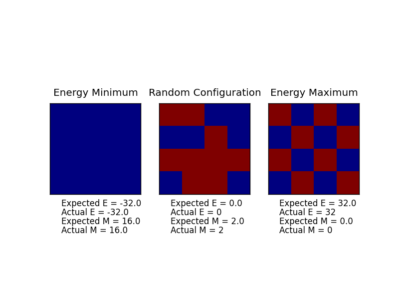
The displayed window has a series of control buttons in the bottom left, one of which will allow you to export the figure as a PNG image. Save an image of the ILcheck.py output, and include it in your report.

The output of ILcheck.py indicates that our code is working:

Introduction to Monte Carlo Simulation

TASK: How many configurations are available to a system with 100 spins? To evaluate these expressions, we have to calculate the energy and magnetisation for each of these configurations, then perform the sum. Let's be very, very, generous, and say that we can analyse $1 \times 1 0^{9}$ configurations per second with our computer. How long will it take to evaluate a single value of ${⟨ M ⟩}_{T}$ ?

The total number of micro-states of the system can be given by: W = n^N, where n is the number of energy levels available to the particles (in our case n=2 as the spins can be 'up' or 'down') and N is the number of particles (in our case, we have N = 100 spins). Therefore, the total number of micro-states of the system = 2¹⁰⁰=1.27*10³⁰.

If we are generous and as we say that we can analyse $1 \times 1 0^{9}$ configurations per second with our computer, it will thus take: 2¹⁰⁰/ $1 \times 1 0^{9}$ = 1.27*10^21 to to evaluate a single value of ${⟨ M ⟩}_{T}$ .

TASK: Implement a single cycle of the above algorithm in the montecarlocycle(T) function. This function should return the energy of your lattice and the magnetisation at the end of the cycle. You may assume that the energy returned by your energy() function is in units of $k_{B}$ ! Complete the statistics() function. This should return the following quantities whenever it is called: $< E >, < E^{2} >, < M >, < M^{2} >$ , and the number of Monte Carlo steps that have elapsed.

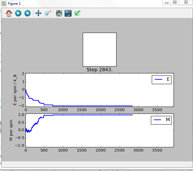
Figure 3: Graphical Outputof ILanim.py: System Converging in Monte Carlo Simulation

Averaged quantities returned: E = -1.78521202942 E*E = 3.34626852553 M = -0.827333946344 M*M = 0.789806648231

TASK: If $T < T_{C}$ , do you expect a spontaneous magnetisation (i.e. do you expect $⟨ M ⟩ \neq 0$ )? When the state of the simulation appears to stop changing (when you have reached an equilibrium state), use the controls to export the output to PNG and attach this to your report. You should also include the output from your statistics() function.

Yes, the Curie temperature is the temperature at which certain magnetic materials undergo a sharp change in their magnetic properties. In our case, the Curie temperature is the temperature above which we will not observe a spontaneous change in magnetization. Below the Curie temperature, as the case above, we will observe a spontaneous change in magnetization.

At low temperatures, the energy term will dominate the free energy equation. Therefore, the most ordered configuration will be favored. At a temperature higher than the Curie temperature, the entropic term will dominate, where average magnetization = 0.

Accelerating the Code

TASK: Use the script ILtimetrial.py to record how long your current version of IsingLattice.py takes to perform 2000 Monte Carlo steps. This will vary, depending on what else the computer happens to be doing, so perform repeats and report the error in your average!

ILtimetrial.py was used 10 times to measure how long the current version of IsingLattice.py takes the to perform 2000 Monte Carlo steps:

7.712165036334581s 7.7131584492012735s 7.7646375205185905s 7.736347742196813s 7.805728469564656s 7.738446858901625s 7.870398107716028s 7.827652376131255s 7.774199458950761s 7.907599321665884s

Average Value: 7.78503333411814s

Standard Deviation = 3.74340219605276s, Standard Error of the Mean: 1.18376771376029s.

TASK: Look at the documentation for the NumPy sum function. You should be able to modify your magnetisation() function so that it uses this to evaluate M. The energy is a little trickier. Familiarise yourself with the NumPy roll and multiply functions, and use these to replace your energy double loop (you will need to call roll and multiply twice!).

NumPy sum, NumPy roll and NumPy multiply functions were used to modify the code (the final Ising Lattice files consists of the modified code).

TASK: Use the script ILtimetrial.py to record how long your new version of IsingLattice.py takes to perform 2000 Monte Carlo steps. This will vary, depending on what else the computer happens to be doing, so perform repeats and report the error in your average!

ILtimetrial.py was again used 10 times to measure how long the modified version of IsingLattice.py takes to perform 2000 Mote Carlo steps:

0.22816197187785292s 0.22886831830965093s 0.2293413289335149s 0.2313109487922702s 0.23568969295683928s 0.23123306957040768s 0.23347285184718203s 0.23241604891518364s 0.2324875891308693s 0.23675011817704217s

Average Value: 0.231973193851081s

Standard Deviation: 0.232413349792457s Standard Error of the Mean: 0.0734955543973584s

Effect of Temperature and System Size

Correcting the Average Code: Experimenting with Different Temperatures and Different System Sizes

TASK: The script ILfinalframe.py runs for a given number of cycles at a given temperature, then plots a depiction of the final lattice state as well as graphs of the energy and magnetisation as a function of cycle number. This is much quicker than animating every frame! Experiment with different temperature and lattice sizes. How many cycles are typically needed for the system to go from its random starting position to the equilibrium state? Modify your statistics() and montecarlostep() functions so that the first N cycles of the simulation are ignored when calculating the averages. You should state in your report what period you chose to ignore, and include graphs from ILfinalframe.py to illustrate your motivation in choosing this figure.

Experimenting with different temperatures

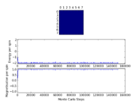
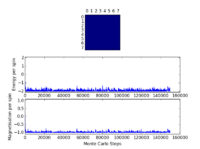
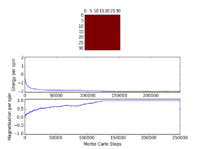
In the table below, we present graphs from ILfinalframe.py obtained at different temperatures (but the lattice size is kept constant at 8x8). The zoomed-in image is shown to identify the approximate number of cycles required for the system to equilibrate. the zoomed-out image is shown to analyze the fluctuations in energy/spin and magnetisation/spin over the larger domain of number of cycles sampled by ILfinalframe.py.

Table 1: Effect of temperature on the number of cycles required for an 8x8 lattice to equilibrate
Temperature (in reduced units of k_B	Variation of Energy and Magnetisation per spin with Number of Cycles of Simulation: Zoomed in Image	Variation of Energy and Magnetisation per spin with Number of Cycles of Simulation: Zoomed Out Image	Approximate number of cycles needed for system to go from its random starting position to the equilibrium state
0.1			500
0.5			500
1.0			1000
1.5			1500
2.0			Reaches a minimum value for energy/spin and magnetisation/spin at around 2000 cycles, but significant fluctuations after this
2.5			Does not equilibrate within 150,000 cycles and significant fluctuations of energy/spin and magnetisation/spin throughout
3.0			Does not equilibrate within 150,000 cycles and significant fluctuations of energy/spin and magnetisation/spin throughout

Effect of temperature:

From the graphs in the table above, we see that an increase in temperature tends to lead towards an increase in the number of cycles required for the system to equilibrate.

Furthermore, we observe that an increase in temperature tends to lead towards an increase in the size of the fluctuations of the energy/spin and magnetisation/spin over the entire domain of the number of cycles.

When the temperature is above 2, the fluctuations in energy/spin and magnetisation/spin are significant throughout the 150,000 cycles sampled. Moreover, the system never converges to the minimum energy value (we can see that the final configuration is not one in which all the spins are aligned). This obviously means that we cannot use graphs corresponding to temperatures above 2 to identify the number of cycles required for the system to equilibrate.

This is again because of the playoff between entropic and enthalpic effects on energy. At higher temperatures, the entropic effect becomes more significant - the tendency for the system to equilibrate to the most stable state decreases.

A Note on Reaching Equilibrium and Ignoring the first N cycles:

When T = 1 k_B, around a 1000 cycles are needed for the system to from its random starting position to the equilibrium state. After a 1000 cycles (the relaxation lifetime), there are a few minor bumps in the energy per spin and magnetization per spin after the system has equilibrated around an average value. We thus need to ignore > he first 1000 cycles when calculating the averages - this author has chosen to ignore the first 2000 cycles.

We can observe the effect of ignoring the first N cycles our simulation (where N > number of cycles typically required to reach equilibrium) by comparing the average values (of E, E², M, M²) before and after ignoring the first N Cycles.

For example, we can compare these sets of values before and after ignoring the first 2000 cycles of a simulation using an 8x8 lattice. Both calculations were done by averaging over approximately 5000 cycles (the ILanim.py program was allowed to run for 5012 cycles for the simulation conducted before IsingLattice was changed, and the program was allowed to run for 7022 cycles for the simulation conducted after IsingLattice was altered to ignore the first 2000 cycles when calculating the average values.

Table 2: Comparison of Average Quantities of Energy and Magnetisation Obtain with and without ignoring the first 2000 cycles
Quantity	Average Value obtained through Monte Carlo Simulation averaging over values from first 5000 Cycles	Average Values obtained through averaging over cycles 2000 to 7000 (ignoring first 2000 cycles)
<E>	-1.78521202942	-2.0
<E²>	3.34626852553	4.0
<M>	-0.827333946344	1.0
<M²>	0.789806648231	1.0

We can see that the values for energy converges to a lower value when we don't take the first 2000 cycles into account. This value is an integer and exactly what we would expect the energy of the lowest energy configuration to be. We thus understand that by ignoring the first 2000 cycles, we are able to much precisely determine the equilibrium values required.

Experimenting with different Lattice Sizes

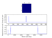
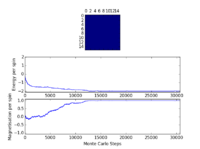
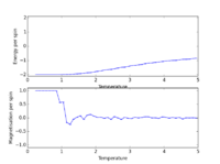
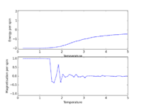
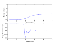
In the table below, we present graphs from ILfinalframe.py obtained using different lattice sizes (but the temperature is kept constant at 1 k_B). The zoomed-in image is shown to identify the approximate number of cycles required for the system to equilibrate. the zoomed-out image is shown to analyze the fluctuations in energy/spin and magnetisation/spin over the larger domain of number of cycles sampled by ILfinalframe.py.

Table 3: Effect of lattice size on the number of cycles required for an 8x8 lattice to equilibrate
Lattice Size	Variation of Energy and Magnetisation per spin with Number of Cycles of Simulation: Zoomed in Image	Variation of Energy and Magnetisation per spin with Number of Cycles of Simulation: Zoomed Out Image	Approximate number of cycles needed for system to go from its random starting position to the equilibrium state
2x2			<50
4x4			500
8x8			1000
16x16			15000
32x32			150000

Effect of increasing lattice size

From the graphs in the table above, we see that an increase in lattice size results in an increase in the number of cycles required for the system to equilibrate. This is because with an increase in lattice size, there are more spins to be aligned (for the system to converge to the lowest energy state) and thus we can expect the system to require more cycles to equilibrate.

Effect of Temperature and System Size

TASK: Use ILtemperaturerange.py to plot the average energy and magnetisation for each temperature, with error bars, for an $8 \times 8$ lattice. Use your initution and results from the script ILfinalframe.py to estimate how many cycles each simulation should be. The temperature range 0.25 to 5.0 is sufficient. Use as many temperature points as you feel necessary to illustrate the trend, but do not use a temperature spacing larger than 0.5. T NumPy function savetxt() stores your array of output data on disk — you will need it later. Save the file as 8x8.dat so that you know which lattice size it came from.

TASK: Repeat the final task of the previous section for the following lattice sizes: 2x2, 4x4, 8x8, 16x16, 32x32. Make sure that you name each datafile that your produce after the corresponding lattice size!

Final datafiles produced:

File:2x2 mine.dat File:4x4 mine.dat File:8x8 mine.dat File:16x16 mine.dat File:32x32 mine.dat

When using ILtemperaturerange, we use temperature spacing of 0.1 for each simulation.

Ignoring the first 'N' Cycles:

When working at sufficiently low temperatures, we should ignore at least the first N cycles that our system typically requires to reach equilibrium when calculating the averages of E, E2, M and M2 to ensure that we only average over values of E, E2, M, M2 obtained after the system has reached equilibrium. In fact, in the next part of this experiment, for all lattice sizes (except 32x32), we will ignore the first N cycles where N is equal to twice the approximate number of cycles required for the system to reach equilibrium as according to Table 3. For the lattice 32x32, we only ignore the first 150,000 cycles itself.

We vary number of cycles of each simulation for each lattice size tested based on intuition, results from ILfinalframe as shown in Table 3 and considering the first N cycles ignored when calculating the averages).

The chosen parameters to test the different lattice sizes are summarized in the table below:

Table 4: Number of cycles ignored when calculating averages of E, E2, M, M2 for various lattice sizes tested
Lattice Size	First N cycles ignored when calculating the averages	Number of cycles in the simulation (Run-time)
2x2	100	50,000
4x4	1000	100,000
8x8	2000	200,000
16x16	30,000	300,000
32x32	150,000	400,000

Error Bars: In our graph, we plot average/mean values of E vs T (averaged over a specified number of cycles sampled). We can calculate the standard error of this value (the standard error of the mean). The standard error of the mean is a measure of the error associated with the calculated average value and can be used to draw the error bars.

The standard error of the mean (SEM) = standard deviation (SD) / sqrt (n)

where n is the size of the sample

SD = sqrt (Variance).

where Var = <E² - <E>²

We use these equations to calculate the SEMs for values of avgE and avgM at various temperaures for the various lattice sizes tested in our Python code (attached above).

Graphs Produced:

Table 5: Plots of Energy/Spin and Magnetisation/Spin vs Temperature for Various Lattice Sizes Tested
Lattice Size	Plots of Energy/Spin and Magnetisation/Spin vs Temperature for Various Lattice Sizes Tested
2x2
4x4
8x8
16x16
32x32

TASK: Write a Python script to make a plot showing the energy per spin versus temperature for each of your lattice sizes. Hint: the NumPy loadtxt function is the reverse of the savetxt function, and can be used to read your previously saved files into the script. Repeat this for the magnetisation. As before, use the plot controls to save your a PNG image of your plot and attach this to the report. How big a lattice do you think is big enough to capture the long range fluctuations?

Energy per Spin vs Temperature: Final Python Code: File:YC Energy per spin vs Temp.txt

Plots of Energy per Spin vs Temperature for Various Lattice Sizes Tested

Magnetisation per Spin vs Temperature: Final Python Code: File:YC Magnetisation per spin vs Temp.txt

Plots of Magnetisation per Spin vs Temperature for Various Lattice Sizes Tested

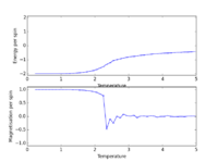
From all the data collected, we can understand that a phase transition occurs somewhere between temperatures of 2 and 3: we observe an inflection point in the energy/spin vs temperature graph and a rapid decrease in magnetisation in the magnetisation/spin vs temperature graph. Near the region of the phase transition, the entropic and energetic terms are now equally important and thus fluctuations over long ranges can occur. From our data, we see that as the lattice size increases, the curves begin to converge.

We can understand that the larger the lattice size used, the more accurately do the plots depict the relationship between energy/spin and magnetisation/ spin vs temperature as an approximation for large, real systems (larger lattice sizes are able to caputre long range fluctuations of the system better).

We see that the 8x8 lattice gives a curve that is already very similar to the curves corresponding to data obtained using the 16x16 and 32x32 lattices. Furthermore, the difference between the curves obtained using the 16x16 and 32x32 lattices is hardly noticeable by eye.

I would say that the 16x16 lattice is big enough to capture the long range fluctuations.

Determining the Heat Capacity

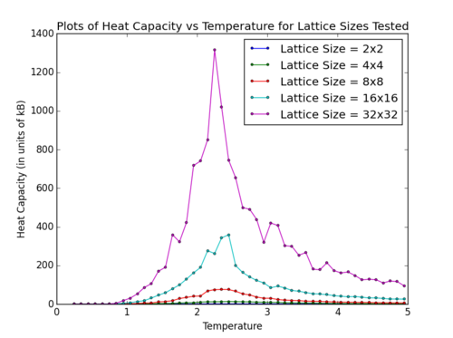
TASK: Write a Python script to make a plot showing the heat capacity versus temperature for each of your lattice sizes from the previous section. You may need to do some research to recall the connection between the variance of a variable, $V a r [X]$ , the mean of its square $⟨ X^{2} ⟩$ , and its squared mean ${⟨ X ⟩}^{2}$ . You may find that the data around the peak is very noisy — this is normal, and is a result of being in the critical region. As before, use the plot controls to save your a PNG image of your plot and attach this to the report.

We use the equation: $C = \frac{\partial E}{\partial T} = \frac{V a r [E]}{k_{B} T^{2}}$

Where the variance of the energy, as aforementioned, is given by:

Var[E] = <E² - <E>²

We can thus calculate the heat capacity and heat capacity/ spin at different temperature for the various lattice sizes tested.

Final Python code for Heat Capacity vs Temperature: File:YC Heat Capacity vs Temp.txt

Plots of Heat Capacity vs Temperature for Various Lattice Sizes Tested

Final Python code for Heat Capacity vs Temperature: File:YC Heat Capacity per spin vs Temp.txt

Plots of Heat Capacity per spin vs Temperature for Various Lattice Sizes Tested

Locating the Curie Temperature

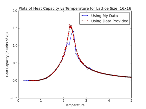
TASK: A C++ program has been used to run some much longer simulations than would be possible on the college computers in Python. You can view its source code here if you are interested. Each file contains six columns: $T, E, E^{2}, M, M^{2}, C$ (the final five quantities are per spin), and you can read them with the NumPy loadtxt function as before. For each lattice size, plot the C++ data against your data. For one lattice size, save a PNG of this comparison and add it to your report — add a legend to the graph to label which is which. To do this, you will need to pass the label="..." keyword to the plot function, then call the legend() function of the axis object (documentation here).

We choose to plot the C++ data against our data of heat capacity per spin vs temperature (as the question does not specify which of E, M or C to plot).

The final files for plotting C++ data and my data on the same graph for different lattice sizes: File:YC Heat Capacity Comparison 2x2.txt File:YC Heat Capacity Comparison 4x4.txt File:YC Heat Capacity Comparison 8x8.txt File:YC Heat Capacity Comparison 16x16.txt File:YC Heat Capacity Comparison 32x32.txt

A graph for one of the lattice sizes (chosen size: 16x16) is shown below:

Plots of Heat Capacity per spin vs Temperature using my data and provided data for 16x16 lattice

TASK: write a script to read the data from a particular file, and plot C vs T, as well as a fitted polynomial. Try changing the degree of the polynomial to improve the fit — in general, it might be difficult to get a good fit! Attach a PNG of an example fit to your report.

Scripts have been written to read and plot the required data from either files containing my data or from the provided files. In both scripts, data corresponding to the 16x16 lattice is used. (This can easily be altered by changing every instance of '16x16' in the files with the desired lattice size).

Plotting C vs T and fitting with polynomial - Using My Data:

File:YC Heat Capacity Fitted My Data 16x16.txt

Polynomial of order 20 appears to give a good fit

Heat Capacity vs Temperature: My Data and Fitted Curve - Lattice Size: 16x16

Plotting C vs T and fitting with polynomial - Using Provided Data: File:YC Heat Capacity Fitted Provided Data 16x16.txt

TASK: Modify your script from the previous section. You should still plot the whole temperature range, but fit the polynomial only to the peak of the heat capacity! You should find it easier to get a good fit when restricted to this region.

Modified Scripts:

Plotting C vs T and fitting peak with polynomial - Using Provided Data:

YC_Heat_Capacity_Fitted_Peak_Provided_Data_16x16_Cmax.txt

Polynomial of order 18 appears to give a good fit

Heat Capacity vs Temperature: Provided Data and Fitted Curve - Lattice Size: 16x16

TASK: find the temperature at which the maximum in C occurs for each datafile that you were given. Make a text file containing two colums: the lattice side length (2,4,8, etc.), and the temperature at which C is a maximum. This is your estimate of $T_{C}$ for that side length. Make a plot that uses the scaling relation given above to determine $T_{C, \infty}$ . By doing a little research online, you should be able to find the theoretical exact Curie temperature for the infinite 2D Ising lattice. How does your value compare to this? Are you surprised by how good/bad the agreement is? Attach a PNG of this final graph to your report, and discuss briefly what you think the major sources of error are in your estimate.

Final files for each lattice size used to calculate temperature at which C is a maximum:

File:YC Heat Capacity Fitted Peak Provided Data 2x2 Cmax.txt

File:YC Heat Capacity Fitted Peak Provided Data 4x4 Cmax.txt

File:YC Heat Capacity Fitted Peak Provided Data 8x8 Cmax.txt

File:YC Heat Capacity Fitted Peak Provided Data 16x16 Cmax.txt

File:YC Heat Capacity Fitted Peak Provided Data 32x32 Cmax.txt

These files were used to create the text files with two columns with data on lattice side length and temperature at which C is a maximum:

YC_Data_Tc.txt

We know that the temperature at which the heat capacity has its maximum must scale according to: $T_{C, L} = \frac{A}{L} + T_{C, \infty}$ , where $T_{C, L}$ is the Curie temperature of an $L \times L$ lattice, $T_{C, \infty}$ is the Curie temperature of an infinite lattice, and $A$ is a constant.

The following file was used to plot 1/L vs $T_{C, L}$ and print the value of the y-intercept ( $T_{C, \infty}$ ):

YC_FinalCurveFit.txt

Plot of: 1/L vs $T_{C, L}$ :

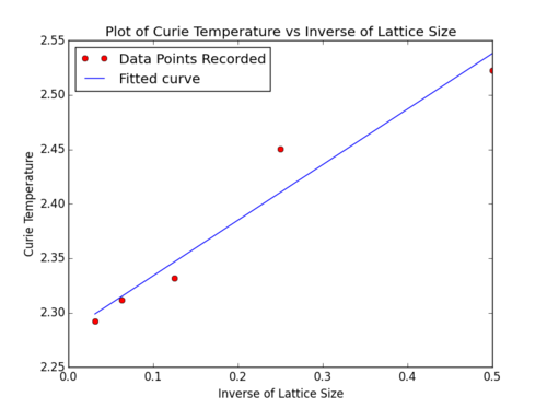
Y-intercept printed: 2.28288746917

Theoretical Exact Curie Temperature: 2.269 ^[1]

Error in our calculated temperature is:

(2.28288746917-2.269)/2.269 = 0.612%

The small error implies that our calculated Tc is reasonably accurate.

Possible Sources of Error:

-> Lattice sizes tested: We saw in the graph: "Plots of Energy per Spin vs Temperature for Various Lattice Sizes Tested", that the larger the lattice size used, the more accurately do the plots depict the relationship between energy/spin and magnetisation/ spin vs temperature as an approximation for large, real systems (larger lattice sizes are able to capture long range fluctuations of the system better). In our final plot used to determine the Tc for infinite lattice, we used data points from the smaller lattice sizes as well (larger 1/L), even though the smaller lattice sizes may not be able to used accurately to determine Tc. The smaller the size of the lattice, the greater the systematic error involved in the corresponding data point (of Tc vs 1/L). If this experiment were to be repeated, data from only large lattice sizes (e.g. lattice sizes larger than 16) would be used.

-> Polynomial fitting: In this experiment, we used fitted the peak of the C vs T curves with a polynomial functions to find Tc. We found that finding the best polynomial function to fit the data by eye is rather difficult. Using a slightly different degree of polynomial would change the value of Tc obtained by a small amount for every lattice size, and thus this factor contributes a small amount to the error of value of Tc for an infinite lattice obtained.

-> Use of Monte Carlo method: In this experiment, we use the Monte Carlo method to find the equilibrium values of E and M for various systems. The method serves as a probabilistic approach to the problem. Therefore, we would yield slightly different data every time we performed a computation. As we are allowing our simulation to proceed to a large number of cycles and only averaging over equilibrium values, the error associated from this source will be very small. However, this source of error would be more significant for shorter simulations.

-> Number of lattice sizes tested: In this experiment, we use the data obtained using 5 lattice points. Although 5 data points were enough to draw a reasonable straight line trend and get a reasonable estimate for Tc for an infinite lattice - using more data points (testing more lattice sizes) would help us better establish the trend.

References

↑ H.A. Kramers and G.H. Wannier, Phys. Rev. 60, 252 (1941) .

[Curie_Temp-1] H.A. Kramers and G.H. Wannier, Phys. Rev. 60, 252 (1941) .

[1]