Rep:Mod:CYN888

Third year simulation experiment

Section 2 - Introduction to molecular dynamics simulation

Task 1: Editing HO.xls File

Calculated the Analytical Column using the Classical Harmonic Oscillator equation: $x (t) = A \cos (ω t + ϕ) .$

The absolute Error was calculated by subtracting the velocity-Verlet solution from the Analytical column. The total energy of the oscillator was calculated using the equations below (where k=1.00):

Task 2: Estimating position of Error Maxima.

Task 3: Different Values of Timestep

Timestep	Energy Change (%)
0.1	0.20
0.2	1.01
0.175	0.81
0.15	0.60

As you can see from the table, the timestep required to ensure the total energy changes by less than 1% is between 0.175 and 0.2.

As you increase the timestep, you are recording less data points and so the total energy will be less accurate. The total energy actually falls slightly as the timestep is increased, however the fluctuations in energy are larger. It is important to monitor the total energy of a physical system because it should remain constant, due to conservation of energy. Large fluctuations are unfavourable and lack accuracy.

Task 4 - Lennard-Jones Interaction

Finding separation $r_{0}$ at which potential is zero:

$ϕ (r_{0}) = 4 ϵ (\frac{σ^{12}}{r_{0}} - \frac{σ^{6}}{r_{0}}) = 0$

$r_{0} = σ$

The force at this separation is zero, since $F_{0} = - \frac{d ϕ (r^{N})}{d r_{0}}$ , and $ϕ = 0$

Equilibrium separation $r_{e q} = σ^{1 / 6}$

Well depth at $r_{e q},$ = $ϵ$

Evaluating integrals:

$\int_{2 σ}^{\infty} ϕ (r) d r = 0.6035$ (4.s.f), $\int_{2.5 σ}^{\infty} ϕ (r) d r = 0.2030$ , $\int_{3 σ}^{\infty} ϕ (r) d r = 0.08210$ .

Task 5 - Water Molecules

Number of molecules in 1 mL of water?

Density = mass/volume, Density of water = $1000 k g m^{- 3}$

Volume of water = $1 m L = 0.000001 m^{3}$

Mass of water = $1000 \times 0.000001 = 0.001 k g = 1 g .$

Moles of water = mass/(molecular mass) = $1 / 18.01528 = 5.55 \times 1 0^{- 2}$ .

Number of Molecules = $6.022 \times 1 0^{23} \times 5.55 \times 1 0^{- 2} = 3.34 \times 1 0^{22} .$

Volume of 10000 Water molecules?

Number of moles of water = $10000 / (6.022 \times 1 0^{23}) = 1.66 \times 1 0^{- 20}$

Mass of water = $1.66 \times 1 0^{- 20} \times 18.01528 = 2.9916 \times 1 0^{- 19} = 2.9916 \times 1 0^{- 22} k g .$ Volume of water = $(2.9916 \times 1 0^{- 22}) / 1000 = 2.9916 \times 1 0^{- 25} m^{3} = 2.9916 \times 1 0^{- 19} m L$

Task 6 - Cubic Simulation Box

In a single timestep, the x and y coordinates of the atom will leave the central simulation box, and hence will have to be replaced by the replica boxes. The z coordinate change will remain in the central box so will not need to be replaced. The atom will end up at point (0.2, 0.1, 0.7), after the boundary condition has been applied.

Task 7 - Reduced Units

$r^{*} = \frac{r}{σ}$

$r = r^{*} \times σ = 3.2 \times 0.34 \times 1 0^{- 19} = 1.088 \times 1 0^{- 9}$

Well depth: Φ = 4 x (8.85 x 10^-12) x ((((0.34 x 10^-9)^12)/((1.088 x 10^-9)^12))- (((0.34 x 10^-9)^6)/((1.088 x 10^-9)^6))))

$T^{*} = 1.5$

$T = T^{*}$ x ε/kB

and since ε/kB = 120, then

$T = 1.5 \times 120 = 180 K$ .

Section 3 - Equilibration

Task 8 - Random Starting position for atoms...

If random starting coordinates are given to atoms, then the atoms could be generated very close together. This might raise the total energy of the simulation leading to inaccuracy.

Task 9 - Lattice spacing and number density.

In simple cubic lattice, the distance between points on the face of the lattice is the same (1.07722), and the volume is $1.0772 2^{3} = 1.2500$ . If there is one lattice point per unit cell, then the lattice point number density is 1/1.2500 = 0.8.

A face centred cubic lattice has 4 lattice points per unit cell. Number density = (lattice points per unit cell)/(total volume of unit cell). (Total volume of unit cell) = 4/1.2 Since the volume of the cubic unit cell = (side length)^3, then (side length) = (4/1.2)^(1/3) = 1.49380

Task 9 - How many atoms..?

Since the face centred cubic lattice contains 4 lattice points per unit cell, if the box we create contains 1000 lattice points (10x10x10), then we would create 4000 lattice points and hence 4000 atoms.

Task 10 - Purpose of LAMMPS Commands

mass 1 1.0 - the mass of atom type 1 is 1.0

pair_style lj/cut 3.0 - Sets the formula that LAMMPS uses to calculate the pair potentials between pairs of atoms. lj corresponds to the Lennard-Jones potentials used to compute potentials, and cut means that the pair of atoms must be within a certain distance of one another to interact. This distance is set to 3.0 and can be smaller or larger than the dimensions of the simulation box.

pair_coeff * * 1.0 1.0 - pair_coeff specifies the pairwise force field coefficient for one or more pairs of atoms. The asterisk sets the coefficients for multiple pairs of atom types, however in this simulation we only have one atom type. Letting N=the number of atom types (N=1 in this simulation), then the asterisk covers all types of atoms from 1 to N. The 1.0 and 1.0 indicate the coefficients epsilon and sigma from the Lennard-Jones potential respectively. These are required to calculate the potential. The number of and meaning of the coefficients depends on the pair style chosen i.e. lj

Task 11 - Which integration algorithm

We should use the Velocity Verlet algorithm since the Verlet algorithm requires the position one timstep before the initla condition, which we cannot specify. By specifying initial position $x_{i} (0)$ and initial velocity $v_{i} (0)$ we are able to calculate the kinetic energy of our system.

Task 12 - Running the Simulation

The purpose of the lines is to set a timestep, and make enough steps to reach an overall simulation time of 100. Each line of code (bold) is analysed below:

### SPECIFY TIMESTEP ###

variable timestep equal 0.001 - variable timestep is assigned value 0.001

variable n_steps equal floor(100/${timestep}) - variable n_steps is equal to the rounded down integer of 100/(the value of the timestep. Simulation time is 100.

variable n_steps equal floor(100/0.001) - this is a print statement

timestep ${timestep} - the timestep is set to the value above

timestep 0.001 - another print statement

### RUN SIMULATION ###

run ${n_steps} - run command to continue the dynamics for a specified number of timesteps, equal to the value of variable n_steps

run 100000 - a print statement

The following code is not used because the number of timesteps required to complete the simulation time has to be worked out by the user. No variables are being used, hence it is not automated.

timestep 0.001 run 100000

Task 13 - Plotting Thermodynamic data

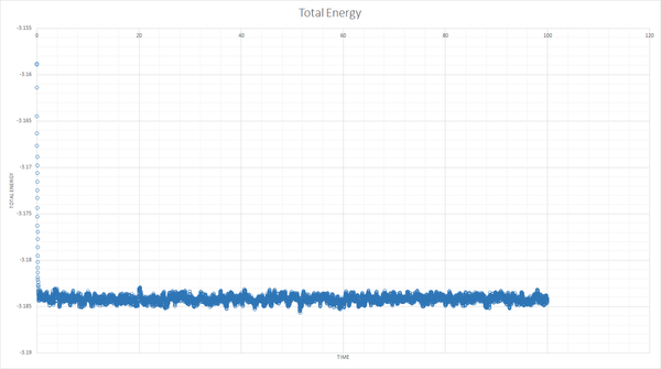
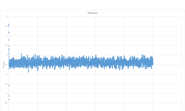
The simulation reaches equilibrium as shown by the total energy, pressure and temperature becoming relatively constant by a time of about 0.5.

Here is a plot of all energies against time, for all of the 5 timesteps used:

The largest timestep to give a suitable result is 0.0025, the yelloe data points. The energy converges to a stable level (to a degree of error), which is much better than the slower timesteps, and of a similar level to to the faster timestep of 0.001 (orange data points).

The particularly bad choice is a timestep of 0.0015 because the energy does not stabilise, and instead it begins to rise. This is due to cumulative error in the energy, and can be seen by the grey data points.

Part 4 -Running simulations under specific conditions

Task 15 - Equations of State

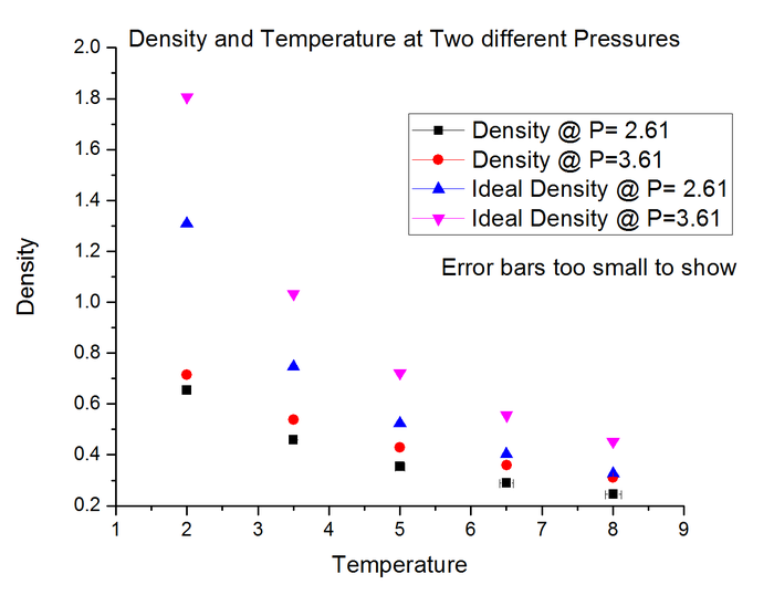
The graph shows plots of density against temperature for two different pressure isobars. The black and red points correspond to the density calculated from the simulation, whereas the blue and pink correspond to density calculated from the ideal gas law.

The simulated density is lower than that from the ideal gas law because it takes into account intermolecular forces between the hard spheres of gas molecules. The molecules therefore repel each other if within a certain distance limit, hence are on average further apart than if no intermolecular interactions were considered (as in the ideal gas law). The discrepancy increases as you increase the pressure, since the molecules are being 'pushed' closer together therefore are interacting more strongly in the simulation. The ideal gas law falls apart when molecules interact more strongly, hence the discrepancy between ideal and simulated density is greater relative to a lower pressure.

Task 16 - Heat Capacity Calculation

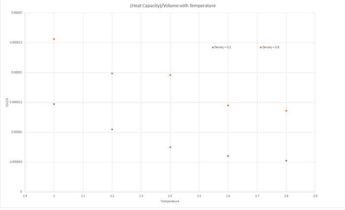
The trend shown in the graph is that as the temperature increases, the Heat Capacity (at constant volume) decreases. Since heat capacity relies on the internal energy of the molecules of the liquid, but is inversely proportional to the change in temperature, then as the temperature increases, the heat capacity will decrease. The Internal energy (U) also increases with temperature, since more excited vibrational and rotational states are created, however this increase is not proportional to the increase of temperature, hence Heat Capacity decreases.

The heat capacity for the greater density is larger for a specified temperature due to the larger density having relatively more internal energy, U.

Input Script for Density = 0.2, Temperature = 2.8:

### DEFINE SIMULATION BOX GEOMETRY ###
variable density equal 0.2
lattice sc ${density}
region box block 0 15 0 15 0 15
create_box 1 box
create_atoms 1 box

### DEFINE PHYSICAL PROPERTIES OF ATOMS ###
mass 1 1.0
pair_style lj/cut/opt 3.0
pair_coeff 1 1 1.0 1.0
neighbor 2.0 bin

### SPECIFY THE REQUIRED THERMODYNAMIC STATE ###
variable T equal 2.8
variable p equal 2.61
variable timestep equal 0.0025

### ASSIGN ATOMIC VELOCITIES ###
velocity all create ${T} 12345 dist gaussian rot yes mom yes

### SPECIFY ENSEMBLE ###
timestep ${timestep}
fix nve all nve

### THERMODYNAMIC OUTPUT CONTROL ###
thermo_style custom time etotal temp press
thermo 10

### RECORD TRAJECTORY ###
dump traj all custom 1000 output-1 id x y z

### SPECIFY TIMESTEP ###

### RUN SIMULATION TO MELT CRYSTAL ###
run 10000
unfix nve
reset_timestep 0

### BRING SYSTEM TO REQUIRED STATE ###
variable tdamp equal ${timestep}*100
variable pdamp equal ${timestep}*1000
fix nvt all nvt temp ${T} ${T} ${tdamp}
run 10000
reset_timestep 0
unfix nvt
fix nve all nve

### MEASURE SYSTEM STATE ###
thermo_style custom step etotal temp press density atoms vol
variable dens equal density
variable dens2 equal density*density
variable temp equal temp
variable temp2 equal temp*temp
variable press equal press
variable press2 equal press*press
variable energy equal etotal
variable energy2 equal etotal*etotal
variable atoms equal atoms
variable volume equal vol
fix aves all ave/time 100 1000 100000 v_dens v_temp v_press v_dens2 v_temp2 v_press2 v_energy v_energy2

run 100000

variable avedens equal f_aves[1]
variable avetemp equal f_aves[2]
variable avepress equal f_aves[3]
variable heatcapacity equal ${atoms}*${atoms}*(f_aves[8]-f_aves[7]*f_aves[7])/(1*f_aves[5]) 

variable errdens equal sqrt(f_aves[4]-f_aves[1]*f_aves[1])
variable errtemp equal sqrt(f_aves[5]-f_aves[2]*f_aves[2])
variable errpress equal sqrt(f_aves[6]-f_aves[3]*f_aves[3])

print "Averages"
print "--------"
print "Density: ${avedens}"
print "Stderr: ${errdens}"
print "Temperature: ${avetemp}"
print "Stderr: ${errtemp}"
print "Pressure: ${avepress}"
print "Stderr: ${errpress}"
print "HeatCapacity: ${heatcapacity}"
print "Volume: ${volume}"

Part 5 - Structural properties and the radial distribution function

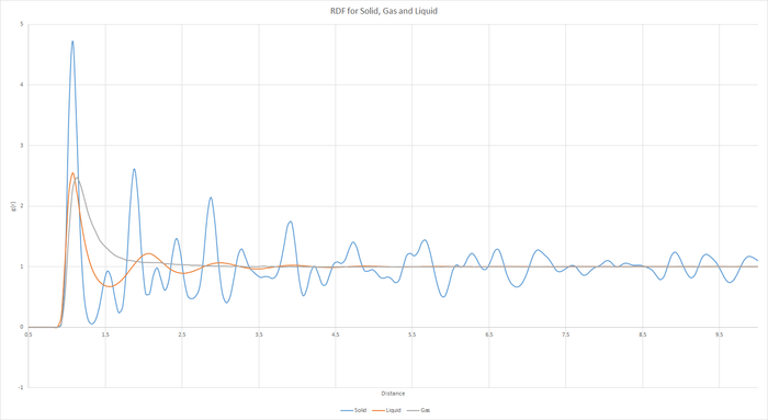
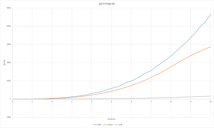
Task 17 - RDF

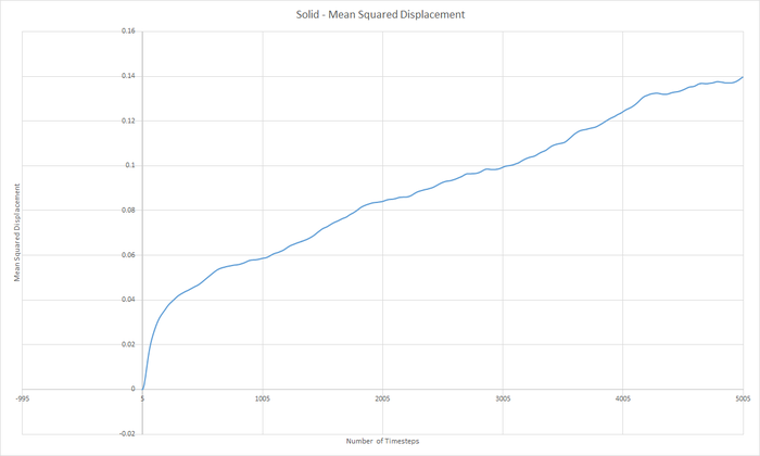
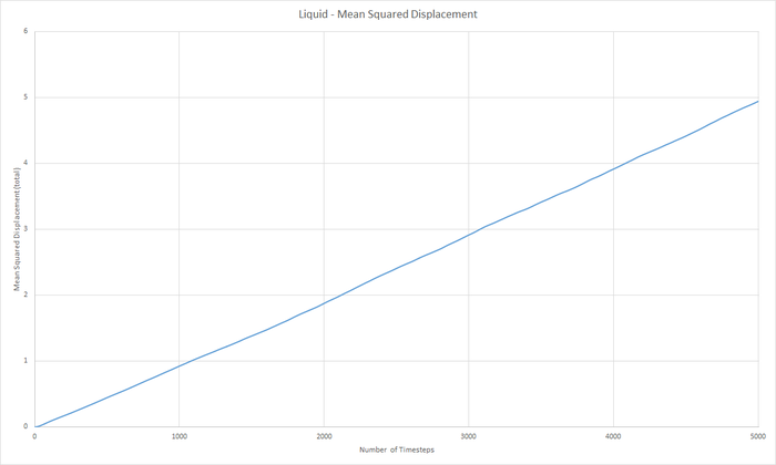
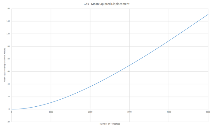
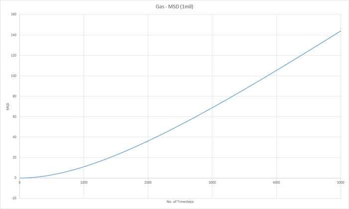
Part 5 - Dynamical properties and the diffusion coefficient Task 18 & 19 - Mean Squared Displacement (MSD)

The diffusion coeffieient, D can be calculated from the slope of the MSD with time graph, divided by 6.

2E-05 1E-03 0.0395