Rep:Mod:CE1014MgO

Thermal Expansion of MgO

Introduction

This investigation involves modelling the thermal expansion of a crystal of MgO, and calculating its thermal expansion coefficient $\alpha$:

$\alpha =\frac{1}{V_0}{\left(\frac{\partial V}{\partial T}\right)}_P$ Eq. 1

Both the Quasi-harmonic Approximation (QHA) and Molecular Dynamics model (MD) are used to calculate the energy and vibrations within the system and therefore compute the thermal expansion coefficient $\alpha$. These approaches are then compared with values found in literature.

In the QHA the crystal is modelled as a collection of quantum phonons. The vibrational energies of the phonons are used to compute the free energy of the crystal at a given temperature, and the volume as a function of temperature is determined. The equilibrium distance between atoms is independent of temperature in the harmonic approximation, which means it cannot describe the thermal expansion of the crystal, whereas the QHA does allow a varying equilibrium distance so is able to model thermal expansion.

The MD simulation uses Newton's classical equations of motion to model the forces and movements of the atoms in the crystal. The physical properties such as free energy and lattice constant are recorded at each time step, and the average of these properties over all time-steps is calculated. The system is assumed to be in equilibrium at some time step when the average temperature over all time steps is close to the value of temperature we have assigned to the computation. At this number of time steps the time averaged properties are recorded.

The crystal structure of MgO in a conventional cell is a face-centered cubic lattice which consists of a total of 8 atoms (Fig 1), it can also be modelled as a primitive cell (Fig. 2); the simplest unit cell, with one ion in the centre and the opposing ion on each corner giving a total of 2 atoms within the lattice. The conventional cell has 4 times the volume of the primitive unit cell however is a more realistic representation of the symmetry of the crystal therefore is still used in many crystallographic studies. In this investigation the primitive cell will be dealt with initially when calculating using the QHA, but a super cell (Fig. 3) is used for the molecular dynamics simulations which is made up of 32 MgO unit cells.

Fig. 1:Conventional cell of MgO

Fig. 2: Primitive cell of MgO

Fig. 3: Supercell of MgO

Method

All calculations were carried out using DLVisualize, a graphical interface used for modelling. Within this programme the modelling code GULP (General Utility Lattice Program) was utilised to calculate the theoretical values evaluated in the Results and Discussion below.

The internal energy, $U$, of the primitive unit cell was initially calculated by modelling the crystal as a purely ionic material which was used in future calculations of the Helmholtz Free Energy ,$A$.

To enable us to visualise how the frequencies of vibrations of this lattice vary with $k$, a phonon dispersion curve was calculated using a sample of 50 k-points and represented graphically (FIg. 4). Subsequently a calculation was run to find the density of states for a lattice grid size of 1x1x1. This calculation was then repeated, doubling the shrinking factor each time until a grid size of 64x64x64 was obtained.

Initially the thermal expansion coefficient was calculated using the QHA:

Using the optimum grid size, found to be 32x32x32 from the above simulations, the Helmholtz Free Energy was found for the MgO crystal at temperatures between 0 K and 1000 K in 100 K intervals. The lattice parameters and the total volume for each cell was recorded at each temperature and plotted.

From the plot of cell volume with respect to temperature, the gradient of the linear section was taken with the initial volume and used in Eq. 1 to give a value of the thermal expansion coefficient, $\alpha$, as $2.64$x$10^{-5}{K}^{-1}$ for a temperature range 400 - 1000 K.

The thermal expansion coefficient was then calculated using Molecular Dynamics.

Within this computation the system has a timestep of 1 femtosecond $(10^{-15}s)$ and runs for 500 steps after equilibrium has been reached at the selected temperature. The same temperature range from 0 K to 1000 K was used as above. The system used was made up of 32 MgO unit cells. The average equilibrium volumes were recorded at each temperature for this simulation.. Eq. 1 was used to calculate the thermal expansion coefficient as above using the gradient of the volume as a function of temperature line of best fit and the initial volume found. Giving a value of $\alpha$ as $2.86$x$10^{-5}{K}^{-1}$ with a temperature range 100 - 1000 K.

Results and Discussion

The internal energy per primitive cell of MgO was found to be -41.0753 eV. MgO was modelled as purely ionic crystal with Mg 2+ ions and O 2- ions having simple Buckingham repulsive potentials operating between the ions, this energy is also described as the 'binding energy' of the crystal as it is the energy necessary to separate the ions to an infinite distance.

The Phonon dispersion curve is shown in Fig. 4 with k-space plotted against frequency of the vibrations.

Fig. 4: Phonon dispersion curve for MgO

The labels on the x-axis are points of interest in k-space. For example the origin is labelled $\mathrm{\Gamma }$ with lattice coordinates [0, 0, 0]. The bands in the phonon dispersion model correspond to the available phonon frequencies at that point in k-space.

To compute the free energy using the QHA, the sum over all vibrations of the lattice is required. To ensure the correct level of accuracy a Density of States (DOS) calculation was run with increasing shrinking factors. The grid sizes used were: 1x1x1 (Fig. 5), 2x2x2 (Fig. 6), 4x4x4 (Fig. 7), 8x8x8 (Fig. 8), 16x16x16 (Fig. 9), 32x32x32 (Fig. 10) and 64x64x64 (Fig. 11).

Fig. 5: Density of states using 1x1x1 grid size

In the initial DOS calculation for the 1x1x1 grid size the graph was computed for a single k-point, corresponding to the point labelled L in k-space with coordinates (0.5, 0.5, 0.5). This can be determined from the examination of the four frequency signals in the 1x1x1 DOS graph (Fig. 5) corresponding to the frequencies that are observed at k-point L on the phonon dispersion graph (Fig. 4), and also read off from the Log file.

• 

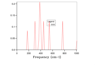
  Fig. 6: 2x2x2

• 

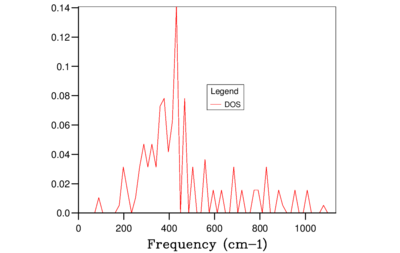
  Fig. 7: 4x4x4

• 

  Fig. 8: 8x8x8

• 

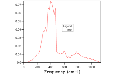
  Fig. 9: 16x16x16

• 

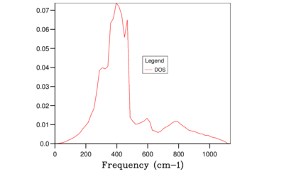
  Fig. 10: 32x32x32

• 

  Fig. 11: 64x64x64

It is clear from the above figures that as the shrinking factor is increasing the accuracy in the Density of States graphs is also increasing. This is due to the number of k-points sampled increasing in each grid size, therefore more phonon frequencies are recorded which increases the smoothness of the graphs. However using this computation method the difference between using a shrinking factor of 32 and a shrinking factor of 64 has very little effect on the shape of the curves, this can be seen in Figure 10 and 11. Therefore the grid size of 32x32x32 was chosen for the calculation of the free-energy of MgO using the QHA as this size being the optimum balance of accuracy and CPU time in this case.

For similar crystal such as CaO, this grid size would also be appropriate as it's lattice parameters are very similar to MgO and they have the same unit cell structure. However for a Zeolite such as Faujasite a smaller grid size would be suitable. This is due to Faujasite having a much larger lattice constant, $a$: 24.638 Å compared to MgO with lattice parameter of 4.216 Å, therefore in reciprocal space the lattice parameter, $a^{*}$ is much smaller and a smaller sample of k-points would give a sufficient degree of accuracy for the DOS calculation. When considering a metal such as Li, the environment of the electrons must be taken into account when determining the necessary grid size for the DOS calculation. In the vibrational structure of a metal, the vibrational bands are much less disperse when compared to the bands of an insulator. This can be explained by the behaviour of the electrons shielding the metal ions as they vibrate within the crystal to minimise the repulsive forces, therefore the electrons do not move as freely and are therefore have less freedom. Thus when calculating the DOS for a metal, a smaller grid size will be suitable as fewer k-points are needed.

An optimum grid size of 32x32x32 was further confirmed when computing the Free Energy of the primitive cell of MgO at 300 K shown in Table 1. As the value for the Helmholtz Free Energy can be said to be converging as grid size increases, the value for the shrinking factor of 64 can be said to be the most accurate. Therefore the Free Energy for the 2x2x2 grid size is accurate to 1 meV and 0.5 meV and the 4x4x4 grid is accurate to 0.1 meV which can be seen from the values in the final column in Table 1. However as a further accuracy can be obtained a larger grid size was preferred and 32x32x32 was chosen as it gave the same value for the Helmholtz Free Energy as 64x64x64 to 6 decimal places without taking as much CPU time.

Table 1

Grid Size	Helmholtz Free Energy (eV)	Difference in Energy from 64x64x64 grid (eV)
1x1x1	-40.930301	3.82x10-3
2x2x2	-40.926609	1.26x10-4
4x4x4	-40.926450	3.30x10-5
8x8x8	-40.926478	5.00x10-6
16x16x16	-40.926482	1.00x10-6
32x32x32	-40.926483	0
64x64x64	-40.926483

Using the Quasi-harmonic approximation the Helmholtz Free Energy, lattice constant,$a$, and cell volume of a primitive lattice of MgO were calculated and recorder at 100 K intervals within the range 0 K to 1000 K (Table 2).

Table 2

Temperature (K)	Helmholtz Free Energy (eV)	Lattice constant (Å)	Cell volume (Å3)
0	-40.901906	2.986563	18.838260
100	-40.902420	2.986563	18.838260
200	-40.909377	2.987604	18.856201
300	-40.928125	2.989390	18.890025
400	-40.958595	2.991629	18.932507
500	-40.999436	2.994134	18.980110
600	-41.049316	2.996820	19.031221
700	-41.107120	2.999643	19.085057
800	-41.171892	3.002587	19.141316
900	-41.243018	3.005634	19.199638
1000	-41.319849	3.008783	19.260042

The value for the Helmholtz Free Energy is becoming more negative as the temperature is increased which is inline with the equation used by the QHA to calculate the Free Energy (F):

$F(T,V)=U\left(V\right)-TS(T,V)$

As temperature, $T$, increases the term $TS(T,V)$ becomes more negative and dominates the equation causing the free energy, $F$ to decrease(Fig. 12). Conversely the lattice constant, $a$, increases with temperature (Fig. 13) as does the volume (Fig.14). The volume of the cell increases with temperature as the higher the temperature the more kinetic energy which can manifest as vibrational energy within the crystal. As this energy increases the amplitude of the crystal vibrations is increasing causing the equilibrium bond length to become greater as the repulsive forces become stronger at shorter distances therefore the distance between the atoms becomes greater. This is the origin of thermal expansion within this approximation.

• 

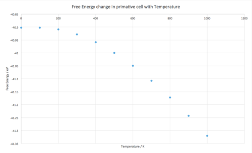
  Fig. 12

• 

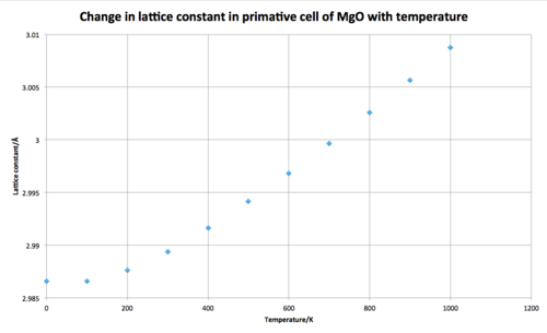
  Fig. 13

Fig. 14

A line of best fit was plotted for the linear region of the data (400 - 1000 K) and its gradient taken for the rate of change of volume with temperature in Eq. 1 and $V_0$ taken as the volume of the cell at 400 K.

$\alpha =\frac{1}{18.932507}0.0005$

$\alpha =2.640960$x$10^{-5}$ $K^{-1}$ (400 - 1000 K)

The thermal expansion coefficient was found using molecular dynamics. This computational approach models the movements of the atoms in the lattice and calculates the thermodynamic properties from the time-averaged behaviour. A supercell made up of 32 conventional lattice cell is used due to the movement of the atoms no longer being periodical therefore more unit cells must be used to model this as accurately as possible. The larger the system in the computation the closer to a real system it becomes and the more accurate the values produced. However due to this computation taking much higher CPU time than when calculating in the QHA only a system of 32 conventional cells were used.

The volume change was plotted against temperature (Fig 15).

Fig. 15

The volume of the system increases linearly, a value for 0 K cannot be calculated for this approximation as MD is based on classical mechanics and does not take into account quantum effects. Therefore at 0 K there would be no kinetic energy and the atom would be at rest; due to the uncertainty principle both the position and momentum of a particle cannot be known simultaneously, and hence the computation breaks down here.

As with the QHA a line of best fit was plotted for the data and its gradient used for the rate of change of volume with temperature in Eq. 1 and $V_0$ the volume at 100 K.

$\alpha =\frac{1}{599.513295}0.0173$

$\alpha =2.885674$x$10^{-5}$ $K^{-1}$ (100 - 1000 K)

Conclusion

Both the Quasi-harmonic approximation (QHA) and the Molecular Dynamics (MD) computations gave values for the thermal expansion coefficient: 2.640960x10^-5 K^-1 and 2.668831x10^-5 K^-1 respectively.

The results for the change in volume per unit cell with respect to temperature is compared for the QHA and for MD Fig. 16.

Fig. 16

When compared with the literature value of 1.140x10^-5 K^-1 (120 - 270) both values give relatively good estimations however the MD result is closer to the literature value.

When in lower temperature ranges the average energy of an atom is smaller and quantum effects become more important. Since QHA takes quantum effects into account by treating the system as a collection of quantum phonons it is more accurate than its classical counterpart - MD computation. We can also get a result for the volume at 0 K as the QHA takes into account the zero point energy. As the temperature increases the QHA breaks down, with its calculation for volume increasing more rapidly with temperature than in the MD case (Fig. 16). The overestimation in volume for the QHA case is due to it neglecting the higher-order anharmonic terms . As the temperature increases the volume in the QHA will continue increasing infinitely as the model does not allow for the breaking of the bonds between the ions and therefore cannot be used near or above the melting point of a crystal. In higher temperature ranges the MD approximation is preferred as it can take into account the breaking of bonds.

Overall, both computational methods are relatively accurate within the temperature ranges considered. It is difficult to say which method is preferred overall as the accuracy varies with the temperature range of the experiment; the QHA approximation working better at lower temperatures and the MD at higher temperatures.

References

- ↑ T.S.Bush, J.D.Gale, C.R.A.Catlow and P.D. Battle, J. Mater Chem., 1994, 4, 831-837
- ↑ W.S. Wise, Am. Miner., 1982, 67, 794-798.
- ↑ II-VI and I-VII Compounds; Semimagnetic Compounds, ed. O. Madelung, U. Rossler and M. Schulz Springer Berlin Heidelberg, Berlin Heidelberg, 1st edn, 1999, vol. 41B, pp 1-6
- ↑ J.M. Ziman, Principles of the Theory of Solids, 2nd Ed. Cambridge University Press, Cambridge, 1972
- ↑ D. Sen, Current Science, 2014, 107, 203-218
- ↑ Goodwin and Mailey, Trans. Amer. Electrochem. Soc. 1906, 9, 96
- ↑ M. Matsui, G. D. Price and A. Patel, Geophysical Research Letters, 1994, 21, 1659 - 1662