Rep:Mod:Am2912p

Module 3: Physical Computational Laboratory

Introduction

Preface

This computational module involves investigating the transition structure/state of a chemical reaction, which represents the molecular geometry that lies at the maxima along the reaction pathway between reactants and products. Once this transition structure has been determined the underlying chemistry of the chemical reaction can be studied, as a consequence a wide field of modern computational chemistry is associated to locating these points along a potential energy surface (PES). In this experiment focuses firstly on the investigation of the the Cope Rearrangement of 1,5-Hexadiene leading onto an in-depth study of two Diels-Alder reactions, all structures will be modeled using GaussView and all subsequent calculations were conducted using the Gaussian program.

Computational Techniques

In practice, the exact mathematical solutions for two body systems are unattainable when investigating large molecules. This is due to the complexity of separating the variables required in order to solve the dynamical equation for the system.. However, recently computational methods have been shown to provide approximate solutions to the dynamical equation, via the use of simplifications/approximations when seperating the variables. A key example is the Born-Oppenheimer Approximation in which the motions of nuclei and electrons are decoupled, this makes it possible to explain the function (Which function? João (talk) 21:27, 16 February 2015 (UTC)) in terms of nuclear positions and generate a PES for the nuclei. This PES can be explored and investigated analytically in terms of the nuclear positions. Transition structures cannot be described by a single energy function (Can't they be described by an energy function of the nuclear coordinates.? João (talk) 21:27, 16 February 2015 (UTC)), as they involve the formation & breaking of bonds, therefore independent particle models must be employed in order to investigate both the the Cope Rearrangement and the Diels-Alder reaction.^[1] The independent particle model assumes that electrons are independent of each other, their interactions are neglected by regarding them as an average property of the whole system (In mean field theories like Hartree-Fock electrons interact with the average charge density generated by other electrons, does this imply electrons don't interact? João (talk) 21:27, 16 February 2015 (UTC)). ^[1] Multiple computational methods are based upon these principles, known as Hartree-Fock theory. Once the method of calculation has been chosen, (ab initio e.g HF or semi empirical e.g AM1) the next decision is to consider the basis set.

The choice of basis set depends on the type of function required to successfully approximate the molecular orbitals to the desired level of accuracy for the specific reaction under investigation. Gaussian itself contains multiple basis sets and many more have been published throughout the literature. A more accurate basis set is comprised of a larger number of functions, however the computational expense of a calculation scales proportionally to the 4th power of the size of the basis set employed, therefore it is essential to find a balance between both computational cost and overall accuracy of the calculation. ^[1] Throughout this investigation multiple methods and basis sets will be used in order to increase the accuracy of the resultant calculations.

The Cope Rearrangement Tutorial

Introduction

Computational chemistry has quickly become an important staple for modelling reactions in order to determine the structure of the reaction's transition state. The first part of this computational investigation studies the [3,3]-sigmatropic Cope rearrangement of 1,5-hexadiene paying particular attention to the conformation of the transition state.

Figure 1: Cope Rearrangement of 1,5-hexadiene

Previous work has been conducted into studying the nature of this reaction mechanism, using computational methods. One example of this is the investigation into whether the reaction proceeds via a biradicaloid or an aromatic transition state.. However this particular investigation will focus on determining the preference of the reaction to proceed via a chair or a boat conformation through investigation into the lowest energy conformations of the transition state structures. Research by Maluendes et al. (1990) determined that the chair transition state was lower in energy than the boat transition state, this investigation will aim to reproduce results which are consistent with this theory.

Optimising the Reactants and Products

Due to the free roation about the multiple C-C single bonds, 1,5 - hexadiene can adopt several possible conformations. Initially a conformer of 1,5-hexadiene with an anti-periplanar linkage was analysed by performing an optimisation calculation,on the cleaned structure, using the Hartree-Fock method, under a 3-21G basis set. The point groups were determined by using the 'Symmetrize' option on the Gaussview interface. Following this a gauche conformer of the 1,5-hexadiene was optimised using the same method, the results of these optimisations are displayed in the table 1 below. These first two optimisations were obtained from initial "guess" conformations, they were subsequently assigned, according to their optimised structure and total energy, to the corresponding conformer in Appendix 1.

Please note: for conversions into kcal mol^-1, a conversion factor of 1 Ha = 627.5 kcal mol^-1 was used.

Table 1: Comparison of HF/3-21G optimised energies for 1, 5 Hexadiene anti & gauche Conformations

Conformation	Structure	Energy/Hartrees HF/3-21G	Point Group
Anti Conformation (anti1) (log file)		-231.69260220	C2
Gauche Conformation (gauche3) (log file)		-231.69266122	C1

By comparing the above energies to those shown in Appendix 1, it can be concluded that the optimised anti conformation is anti1 and the gauche conformer is equivalent to gauche3 the lowest energy conformation.

Predicting the preference between the Anti and Gauche conformers is rather difficult to make and is dependent upon multiple factors, such as Van der Waals attractions/ Pauli repulsions and orbital interactions. These are difficult to predict and quantify without computational techniques.

Contrary to what was expected the most stable conformation (predicted via the HF/3-21G method) is the gauche3 conformer. This result is surprising and goes against the previous calculations by by H. Rzepa, that in the case of butane, the antiperiplanar conformation is approximately 2 k cal mol^-1 more stable than the corresponding gauche conformation (optimised via the 6-311G(d,p) DFT method). The reason for this difference in energy could be due to the amplified Van der Waals attraction in the more electron-rich hexadiene species, or the more likely reason can be attributed to a computational error arising from the use of the lower level (less accurate) HF/3-21G method and basis set, which was employed in the above energy calculations. The HF/3-21G method neglects electron correlation effects, this could be the main reason why this method does not yield the correct global minimum conformation for 1,5-hexadiene.

In addition to this, standard organic chemistry would predict that the anti conformation would lie lower in energy relative to the gauche due to the presence of the 180 degree dihedral angle between the carbon atoms along the hydrocarbon chain. Contrary to what was expected, the gauche 3 conformation obtained possesses a more negative energy value and hence, according to this computational optimisation, exhibits higher stability with respect to the anti 3 conformation. This apparent anomaly has been attempted to be rationalised by Rocque et al who suggests that stabilising hydrogen bonding between the vinyl hydrogen's and the pi electron clouds of the hydrocarbon chain, are enough to stabilise the gauche conformer relative to the anti. However multiple sources have also reported that, as one would expect, the anti conformer is indeed the most stable, thus one would remain skeptical when confirming this by a computational calculation, due to the level of approximation which is inherent to this type of chemistry. However, to allow an effective comparison with the results obtained by H. Rzepa, the most stable conformers of 1,5- Hexadiene would be subjected to approximately the same level of computational analysis, by repeating the optimisation calculation, this time using a DFT/B3LYP method, under a 6-31G* basis set. It was hoped that the using this more comprehensive method of optimisation would yield more accurate results (Did you actually do the comparison for different conformers? João (talk) 21:27, 16 February 2015 (UTC)). The figure below displays the two conformations in their respective Newman projections:

Figure 2.Newman projections of the gauche3 & anti2 conformers of 1,5-hexadiene.

Following Appendix 1 the C_i anti2 conformation of 1,5-hexadiene was drawn and optimised using the same HF/3-21G method outlined above;

Table 2: HF/3-21G optimised energies for 1, 5 Hexadiene anti2 Conformation

Conformation	Structure	Energy/Hartrees HF/3-21G	Point Group
Anti2 Conformation (log file)		-231.69253516	Ci

Both the calculated energy value (-231.69253516 Ha) and the point group (C_i) compare favourably with the value quoted in the appendix (-231.69254 Ha), indicating that the correct conformer was successfully drawn and optimised. Having identified this conformer further optimisation was conducted by reoptimisation at the B3LYP/6-31G* level. It was expected that the more comprehensive optimisation method would yield a more accurate set of results.

Table 3: DFT/6-31G* optimised energies for 1, 5 Hexadiene anti2 Conformation

Conformation	Structure	Energy/ a.u	Point Group
Anti2 Conformation (log file)		-234.61170127	Ci

The geometries of the DFT-optimised conformers were very similar to those optimised by the Hartree-Fock method, however the DFT optimisation yields a lower energy value (-234.61170127 a.u) compared to (-231.69253516 a.u) indicative of a more accurate optimisation, yielding a more energetically stable representation of the conformer. (Is your energy lower because you found a lower energy conformer or because your method yields a lower energy? In general you cannot compare absolute energy values obtained with different methods, as they often use different reference energies. João (talk) 21:27, 16 February 2015 (UTC))

In order to confirm that the HF-method employed was coherent with the results presented in Appendix 1, all possible conformations of 1, 5 Hexadiene were optimised and are presented below. The lowest energy conformer was confirmed to be the gauche3 structure, suggesting that the previously mentioned stabilising hydrogen bonding between the vinyl hydrogen's and the pi electron clouds of the hydrocarbon chain do indeed lead to an overall stabilisation of the conformer.

Table 4: Comparison of HF/3-21G optimised energies for each possible 1, 5 Hexadiene Conformation

Conformation	Structure	Total Energy/Ha	Point Group	Relative Energy/kcalmol-1
gauche1		-231.68771615	C2	3.103
gauche2		-231.69166702	C2	0.624
gauche3		-231.69266122	C1	0.000
gauche4		-231.69153035	C2	0.710
gauche5		-231.68961572	C1	1.911
gauche6		-231.68916016	C1	2.197
anti1		-231.69260220	C2	0.037
anti2		-231.69253516	Ci	0.079
anti3		-231.68907067	C2h	2.253
anti4		-231.69097048	C1	1.060

Table 4, above, does indeed agree with the results cited in Appendix 1. The gauche3 conformation was found to be the most stable and all relative energies were calculated compared to this structure, however it should be noted that due to the relative closeness of these energy values approximations/errors inherent in the calculations could lead to a reorganisation of the most stable energy conformer if a different method/basis set was employed.

Infrared Analysis of the anti2 conformation

In order to further confirm the success of the DFT method a frequency calculation (at the same level) was conducted on the previously optimised structure and the low/negative frequency modes of vibration were subsequently analaysed:

Figure 3: IR Data for DFT anti2 Conformer.

No negative (imaginary) vibrational modes were present in the vibrational data for any of the DFT-optimised anti2 conformation, indicating that the structure has been successfully optimised to a minima (as opposed to a transition state maxima, which would produce a negative vibrational frequency). The simulated Infrared spectrum for the Anti 2 conformation is shown below in Figure 4 .

Figure 4: IR spectrum of anti2 conformation

It is important that no imaginary frequencies were found, the fact that all frequencies are positive confirms that a minima along the PES surface has been found, the frequencies are second derivatives and thus positive values confirm that a minima has been computed. A single imaginary frequency would correspond to a transition state along the reaction co-ordinate whilst three (Why 3? What about 4? João (talk) 21:27, 16 February 2015 (UTC)) imaginary frequencies would correspond to a maxima anywhere on the PES.

Thermochemical Analysis of the anti2 conformation

In addition to the vibrational information, the frequency analysis also provides a breakdown of energy data under the thermochemistry section of the log file. The thermochemical energy parameters calculated are defined below:

Sum of electronic and zero point Energies (ε_o + ε_ZPE): The total electronic energy + the zero point vibrational energy.

Sum of electronic and thermal Energies (ε_o + E_tot): The total electronic energy + the total internal thermal energy, which consists of translational,rotational and vibrational energy contributions.

Sum of electronic and thermal Enthalpies (ε_o + H_corr): The total electronic energy + the correction to the enthalpy due to internal energy.

Sum of electronic and thermal Enthalpies (ε_o + G_corr): This is the total electronic energy + the Gibbs free energy due to internal energy. (Any idea how the entropy would be calculated in this case? João (talk) 21:27, 16 February 2015 (UTC))

Table 5. Thermochemistry data at 298.15K
Zero-point correction=                                0.142490 (Hartree/Particle)
Thermal correction to Energy=                         0.149846
Thermal correction to Enthalpy=                       0.150790
Thermal correction to Gibbs Free Energy=              0.110886
Sum of electronic and zero-point Energies=           -234.469211
Sum of electronic and thermal Energies=              -234.461855
Sum of electronic and thermal Enthalpies=            -234.460911
Sum of electronic and thermal Free Energies=         -234.500815

Re-calculation at 0K

Gaussian can also calculate these thermochemical corrections at different temperatures, the information above was recalculated at 0K log file

Note: It was found that setting the temperature to 0K caused the calculation to fail, therefore 0K was defined as 0.0001K in the Gaussian input file.

Table 6. Thermochemistry data at 0.0001K
Zero-point correction=                                0.142927 (Hartree/Particle)
Thermal correction to Energy=                         0.142927
Thermal correction to Enthalpy=                       0.142927
Thermal correction to Gibbs Free Energy=              0.142927
Sum of electronic and zero-point Energies=           -234.468774
Sum of electronic and thermal Energies=              -234.468774
Sum of electronic and thermal Enthalpies=            -234.468774
Sum of electronic and thermal Free Energies=         -234.468774

These results show that at 0K the sums of all the energy and enthalpy parameters are equal in comparison to 298.15K where there is a clear difference between four different energies and enthalpies. This is coherent with theory, at 0K there is no thermal contribution to the energies therefore, only the total electronic energy (and zero point energy) is considered for each of the calculated parameters.

By comparing these results to that at 298.15K it can be seen that the the total energies and enthalpies which include the thermal terms tend to increase (become more positive), despite the free energy correction parameter decreasing with increased temperature. This is also to be expected and is rationalised by the Gibbs Free Energy equation: G = H - TS. Increasing the simulated temperature decreases the the total Gibbs Free Energy of the system, as the entropic contribution is amplified at higher temperatures.

Optimising the "Chair" and "Boat" Transition Structures

Having optimised the reactants and therefore the products of the Cope rearrangement of 1,5-hexadiene, the next step was to investigate the transition state between these. As previously mentioned, the Cope rearrangement can occur via one of two transition states, the chair or the boat transition state.

The structures of the transition states can be predicted from the constituent allyl (CH₂CHCH₂) fragments. Prior to analysing the transition state the allyl fragment was modeled and optimised. Owing to the simplistic nature and small size the allyl fragment can be sufficiently optimised using the HF method under a low level 3-21G basis set. (For our purposes this is true, however we could be interested in high precision measurements, spectroscopy or otherwise. João (talk) 21:27, 16 February 2015 (UTC))

The optimised structure of this fragment is displayed in figure 5 below. The LOG file for this optimisation can be found here.

Figure 5. HF/3-21G optimised allyl fragment

Optimising the "Chair"

Two optimised allyl fragments were arranged in such a way to form a pseudo-chair transition state conformation, shown in Figure 6 below. The interatomic distance between the two terminal carbon atoms of each allyl fragments was set to 2.2Å and the C_2h point group was confirmed.

Figure 6 C_2h Chair transition state after initial optimisation.

This pseudo-transition state was then subjected to two separate methods of optimisation: The first method (a) involves computing the Hessian matrix, which is updated with each optimisation, whilst the second method (b) requires the reaction coordinate to be frozen whilst the rest of the molecule is optimised, followed by subsequent unfreezing of the reaction coordinate and optimiation to a transition state. Method (b) is generally employed to larger systems, as the initial freezing and unfreezing of the reaction coordinate produces a reasonable 'first guess' of the Hessian matrix (It is not so much that the guess for the Hessian is better, but that we only need to calculate force constants along the hypothesized reaction coordinate instead of the full molecule. João (talk) 21:27, 16 February 2015 (UTC)), and therefore can significantly reduce the time taken for the fully optimised Hessian matrix to be calculated.

Method (a): The pseudo-chair structure was optimised to a transition state by computing the Hessian matrix at each step in the optimisation. This was achieved by selecting Optimise to a TS(Berny), using the HF method under a low level 3-21G basis set.

The resultant log file for this optimisation can be found here. It was noted interatomic distance between the two sets of terminal bonding carbon atoms had decreased from (preset) 2.20Å to 2.02Å.

The frequency analysis performed during this optimisiation displays the single characteristic imaginary frequency at -818cm^-1 (intensity = 5.87)corresponding to the Cope rearrangement. This confirms that the model had been successfully optimised to a transition state, as opposed to an energy minimum, where no imaginary frequencies are present.This is extremely important and confirms that we have indeed found a transition state, as opposed to a minima/maxima on the PES. The single imaginary frequency corresponds to a second derivative confirming that a maxima has been reached on the PES which is along the reaction co-ordinate, if multiple imaginary frequencies were present this would simply indicate that a maxia somewhere on the PES was located and not along the reaction coordinate. This singular imaginary frequency also corresponds to the bond forming/breaking vibration which occurs at the transition state, therefore a visual animation of this single frequency will be displayed for each optimised transition state in order to confirm that this mode has been successfully computed. An animation of this negative vibrational mode is shown in figure 7:

Figure 7 Animation of the imaginary frequency corresponding to the Cope rearrangement using method (a)

Method b): The pseudo-chair structure was then optimised to a transition state by using the 'frozen co-ordinate method', which requires two optimisation steps (the first to freeze the reaction co-ordinate and optimise the rest of the structure and the second to optimise to a transition state, as in method (a)).

Using the Redundant Co-ordinate Editor, from the edit menu, and freezing the co-ordinates between the two sets of terminal carbon atoms the system was optimised, resulting in an initial structure where the interatomic distance between the two sets of terminal bonding carbons atoms was frozen at 2.20Å. This system was then optimised to a minimum using the HF method under a low level 3-21G basis set, similar to method (a). The resultant log file for this optimisation can be found here. It should be noted that, the interatomic distance between the two terminal carbon atoms of the allyl fragments that were to undergo bonding had decreased to 2.02Å as with the normal Hessian matrix method (a). The frequency of the imaginary vibration was very similar to the value obtained for the Hessian matrix method (a), again rounding to -818cm^-1, with the slightly lower intensity of 5.83. This singular imaginary frequency again confirms that the structure had been optimised to a transition state, as opposed to minimum. An animation of the synchronous negative vibrational mode is shown below:

Figure 8 Animation of the imaginary frequency corresponding to the Cope rearrangement using method (b)

In this example both methods are successful in optimising to a a transition state and give internuclear distances (2.02Å) which are consistent with literature values using the same low level 3-21G basis set.

Optimising the "Boat"

Following succesful optimisation of the chair transition state the next step in this investigation was to study the boat transition state. Due to the nature of this transition state a different method must be used (Wouldn't previous methods have worked in this case? João (talk) 21:27, 16 February 2015 (UTC)), namely the QST2 method. The success of the method is heavily dependent on both the inital and final structures of the reactanats and products, namely the difference between these two forms.

The anti2 conformation was determined to be the reactant molecule. In order for the QST2 method to be successful the reactant and product molecules must be labelled as in figure 9 below.

Figure 9: Image of the labelled fragments for the boat conformation

After renumbering the product an initial QTS2 Gaussian calculation was conducted. This initial optimisation failed, it did not produce in the desired transitions state, instead the result was a valid chair transition state. For a successful QST2 calculation the reactants and products must bear some structural resemblance to the transition state. In this case the two fragments were unable to rotate about the central C-C bonds to produce the correct structure. Therefore the geometry of the fragments had to be altered manually to allow the transition state to be constructed. The dihedral angle along the four carbon backbone of both structures was changed to 0^o, and the triatomic C-C-C angle between the three 'inner' carbon atoms was reduced to 100^o. This yielded the desired boat transition state:

Figure 10: Image of the altered geometry fragments for the boat conformation

An optimisation under the QTS2 method was performed, which yielded the following boat transition state, log file found here.

The interatomic distance between the two bonding ends of the transition state was determined to be 2.14Å. The frequency of the imaginary vibration was observed at -840cm-1, with the intensity of 1.62. This singular imaginary frequency indicates that the structure has been successfully optimised to a transition state, as opposed to a minimum. An animation of this vibrational mode is displayed below:

Figure 11 Animation of the imaginary frequency corresponding to the Cope rearrangement for the boat transition state

Optimising the Boat Transition Structure using QST3

In addition to the QST2 method employed above, there is another method for optimising the boat transition state, namely the QST3 method. This method allows the user to input the geometry of a guess transition structure and has been known to produce more reliable results. Starting from the two anti2 conformers and a guess transition structure a QST3 calculation was conducted, interestingly in stark contrast to the initial QST2 method this calculation did not fail and successfully produced a boat transition structure. The figure below depicts the input for the QST3 calculations, the third pane shows the "guess" transition structure:

Figure 12 QST3 input structures.

The resultant transition state structure displays the correct atom labeling in regards to both reactant and product molecules, upon comparison with the structure produced via the QST2 method it was noted that the QST3 computation yielded a boat transition structure with a slightly different geometry, this is displayed in the table below:

Table 7. Comparison of QST2 and QST3 Boat Transition Structures.

Atom Labels	QST2 bond length (Å)	QST3 bond length (Å)
C3-C4	2.13999	2.13984
C2-C5	2.77960	2.77944
H8-H12	2.19230	2.19223

Table 8: Comparison of QST2 & QST3 optimised boat transition structure

Optimisation Method	Total Energy/Ha	RMS Gradient
QST2	-231.60280249	0.00000523
QST3	-231.60280236	0.00003049

Due to the extremely similar values for the total energy it can be implied that the same transition structure has been found via each optimisation method, although this goes against the data obtained for the relative geometries of each structure (Why against the structural data. The structures seem to differ very little. Any idea on how the small differences you obtained could be made even smaller? João (talk) 21:27, 16 February 2015 (UTC)). The resultant structure for the QTS3 computation is shown below and the log file for this optimisation can be found here.

Figure 13 Diagram of the QST3 Boat Transition State

In order to confirm that this was indeed a transition state, as opposed to a minima, a frequency analysis was conducted. Due to the presence of a single imaginary frequency (-840 cm^-1) it was confirmed that the QST3 method had indeed produced the expected boat transition state successfully, an animation of this vibration is shown below, the movement is identical to that produced under QST2, showing the bond-forming motion in an asynchronous manner:

Figure 14 Animation of the imaginary frequency corresponding to the Cope rearrangement for the QST3 boat transition state

Intrinsic Reaction Coordinate (IRC) Calculations

Results obtained in the previous section from HF-optimisations of the two transition states is insufficient in determining which conformation of 1,5- Hexadiene the transition state collapses into. However, it is possible to run an Intrinsic Reaction co-ordinate which follows the minimum energy pathway from a transition state down to its local minimum on the potential energy surface, by making small changes to the geometries along the steepest gradient/slope of the energy surface. In general IRC calculations provide a useful and efficient method for exploring the PES of the desired system.

Chair IRC Anlaysis

50 Step Optimisation:

The initial IRC calculation was performed by computing 50 points along the intrinsic reaction coordinate, corresponding to the collapse of the chair transition state, in the forward direction only. The LOG file for the resultant structure that was returned from this calculation can be found here.

The table below displays a summary of results for the output structure:

Table 9: Results Summary for 50 Step IRC Calculation of the Chair Conformation

Total Energy/Ha	RMS Gradient	Number of Intermediates
-231.68515	0.00146725	20

The IRC calculation produces two different graphs, the first Figure 15 displays the variance of Total Energy versus the Intrinsic Reaction Coordinate.

Figure 15: Total Energy Graph for 50 step IRC Optimisations of the Chair Configuration

The second graph Figure 16 plots the variance of the RMS Gradient versus the Intrinsic Reaction Coordinate.

Figure 16: RMS Gradient Graph for 50 step IRC Optimisations of the Chair Configuration

It is clear from the plots above that the optimisation calculation is not entirely complete, whilst the energy has tended towards a minimum the RMS gradient had not yet reached zero. In order to correct for this three separate methods were investigated to complete the calculation:

i) A HF/3-21G optimisation was performed on the structure corresponding to the final data point on the graphs (Structure 44)

ii) The optimisation was repeated, but this time taking 100 data points along the reaction coordinate, as opposed to 50.

ii) The optimisation was repeated, but this time re-calculating the force constant at every step.

i) Normal Minimisation from Final Intermediate of 50 point IRC method:

The first optimisation method required the final structure corresponding to the final data point to be minimised under a normal HF/3-21G energy optimisation. The LOG file for the resultant structure from this method can be found here and is modeled in the following link.

Table 10: Results Summary for Normal HF/3-21G Optimisation

Total Energy/Ha	RMS Gradient
-231.69167	0.00000474

ii) 100 Step Optimisation:

The second method involved performing the same IRC calculation but this time computing 100 data points instead of 50, although this resulted in both a slightly lower total energy and RMS gradient norm, the values were not comparable to any conformations in Appendix 1, the log file for this optimisation can be found here. (I'm puzzled by this observation. How does the structure compare to the different minima? João (talk) 21:27, 16 February 2015 (UTC))

Table 11: Results Summary for 100 Step IRC Optimisation of the Chair Conformation

Total Energy/Ha	RMS Gradient
-231.61932	0.00005817

iii) 50 Step Optimisation, calculating Force constants at every step:

The final optimisation method involved calculating the force constants at every step, which produced the following log file found here.

Interestingly this optimisation went through 44 intermediates, over twice the amount produced by the IRC method calculating the force constants only once. The results summary for this IRC optimisation is shown below:

Table 12: Results Summary for 50 Step IRC Optimisation (calculating the force constant at every step)

Total Energy/Ha	RMS Gradient	Number of Intermediates
-231.69158	0.00015225	44

Figure 17: Total Energy Graph for 50 step IRC Optimisations of the Chair Configuration

Figure 18: Total Energy Graph for 50 step IRC Optimisations of the Chair Configuration

In addition to the increased number of observed intermediates, the value for the RMS Gradient has decreased by approximately two orders of magnitude. Suggesting that the geometry has been optimised to a greater extent compared to method ii).

By comparing both the total energy and RMS gradient values for methods i) to iii) it can be seen that method i) yields the most successfully optimised structure, with the lowest RMS gradient and an energy value which directly corresponds to the gauche2 conformation presented in Appendix 1.

Boat IRC Anlaysis

The boat transition state was analysed in the same way as outlined above, the most effective method i) was used to minimise the initial IRC calculation, the results of this initial IRC optimisation are shown below and the log file can be found here.

Table 13: Results Summary for 50 Step IRC Optimisation (calculating the force constant at every step)

Total Energy/Ha	RMS Gradient	Number of Intermediates
-231.68471	0.00055246	51

Figure 19: Total Energy Graph for 50 step IRC Optimisations of the Chair Configuration

Figure 20: Total Energy Graph for 50 step IRC Optimisations of the Chair Configuration

Optimisation to a minimum using the normal HF/3-21G method yielded a transition state resembling the gauche3 conformer, again the log file can be found here. The following table compares both the energy and point group of the chair and boat transition states to the respective conformers given in Appendix 1.

Table 14: Comparison of IRC calculations to appendix 1 conformers

Type of Transition state	Energy of IRC calculation (a.u.)	Point group of IRC calculation	Corresponding conformer	Energy of conformer in appendix 1 (a.u.)	Point group of conformer in appendix 1
Chair	-231.69166702	C2	Gauche2	-231.69167	C2
Boat	-231.69266122	C1	Gauche3	-231.69266	C1

Activation Energy Calculations

In order to compare the low level HF/3-21G level to the higher level DFT B3LYP/6-31G* method both the Chair and Boat Transition Structures were subjected to optimisation at the DFT level of theory (How do the DFT optimized structures compare with the HF ones? Do they correspond to transition states? João (talk) 21:27, 16 February 2015 (UTC)), these molecules were subsequently analysed by studying the thermochemistry section of each log file. This allowed for the activation energies of both the transition states to be calculated and compared at both the DFT B3LYP/6-31G* and HF/3-21G levels. In addition to this, the activation energies of both transition states were calculated at two different temperatures; room temperature (298.15K) and absolute zero (0K, again simulated at 0.0001K in order to avoid failure of the calculation.) (Did you actually need this 0K calculation? Couldn't you have obtained the relevant data from the finite temperature thermochemistry section? João (talk) 21:27, 16 February 2015 (UTC))

Tables 14 & 15 below display the different energy values needed to calculate the overall activation energy, at each level of theory and temperature.

Activation energies (at 298.15K) were calculated by subtracting the Sum of the Electronic and Thermal Energies for the anti2 conformer from the Sum of the Electronic and Thermal Energies for the appropriate transition state.

Activation energies (at 0K) were calculated by subtracting the Sum of the Electronic and Zero point Energies for the anti2 conformer from the Sum of the Electronic and Zero point Energies for the appropriate transition state.

Table 15: Summary of Energy (in Hartrees) Results

	HF/3-21G			B3YLP/6-21G*
	Electronic Energy	Sum of Electronic and Zero-Point Energies	Sum of Electronic and Thermal Energies	Electronic Energy	Sum of Electronic and Zero-Point Energies	Sum of Electronic and Thermal Energies
		at 0 K	at 298.15 K		at 0 K	at 298.15 K
Chair TS	-231.619322	-231.466705	-231.461345	-234.554484	-234.411639	-234.405179
Boat TS	-231.602803	-231.450929	-231.445300	-234.540452	-234.398494	-234.392567
Reactant (anti2)	-231.692535	-231.539539	-231.532566	-234.611701	-234.468774	-234.461855

HF/3-21G anti2 log file here B3LYP/6-31G* anti2 log file here HF/3-21G anti2 0K log file here B3LYP/6-31G* anti2 0K log file here

Note: All log files for the chair/boat transition state have been linked previously.

Using the relationships previously stated and the conversion factor (1 hartree = 627.509 k cal mol^-1 the activation energy was calulcated and compared below:

Table 16: Summary of Activation Energies (all energies in kcal^-1 )

	HF/3-21G		B3YLP/6-21G*		Expt.
	at 0 K	at 298.15 K	at 0 K	at 298.15 K	at 0 K
ΔE Chair	45.70	44.69	35.85	35.56	33.5 ± 0.5
ΔE Boat	55.60	54.76	44.10	43.48	44.7 ± 2.0

The main observation from the results above is that the activation energies calculated at the higher level of optimisation (DFT) are much closer to the stated literature values, in the Results Table. This demonstrates that, as expected, lower level methods, such as the primitive Hartree-Fock method, are not suited towards determining activation energies accurately in comparison to the higher level DFT method.

The Diels-Alder Cycloaddition

Introduction

The second section of this module investigates the structures of the transition states for two separate classic Diels-Alder cycloaddition reactions. The Diels-Alder reaction is an example of π₄s + π₂s cycloaddition reaction, in which the π-orbitals of a (generally electron defecient) dienophile species interact with the π-orbitals of a (typically electron rich) conjugated diene. This interaction results in the formation of two new σ bonds between the two species. Furthermore, the reaction is known to occur in a concerted fashion, via a single transition state. In the following investigation two reactions will be analysed: the first ethene with cis-butadiene and finally maleic anhydride with cyclohexadiene.

Investigation into the Cycloaddition of Ethene and cis- Butadiene

Optimising the Reactants

Similarly to the Cope rearrangement investigation above, the first step in simulating the transition state requires optimisation of the reactants. Both of the reactants were drawn in GaussView, and optimised using the semi-empirical AM1 method. This method is more accurate than the Hartree-Fock methods used previously (How did you make this assessment? João (talk) 21:27, 16 February 2015 (UTC)), but less accurate than the DFT-B3LYP/6-31G* method.

cis-Butadiene

During the first step of this investigation a molecule of cis-butadiene was constructed within gaussview and subsequently optimised at both the semi-empirical/AM1 level and at the higher level of theory using the B3LYP/6-31G*method.

Interestingly the semi-empircial/AM1 method prodcued a planar structure whilst the high level basis set produced a bent structure where the dihedral angle was no longer 0 degrees. This bent structure does agree with structures reported in the literature which suggest that the steric hindrance between the the terminal CH₂ groups makes the planar structure more energetically unfavorable. However for the purpose of this investigation a bent structure is not useful, as studying the molecular orbitals requires a high degree of symmetry for these simple calculations (Although the analysis would be slightly more complicated, one could pursue the same study with the distorted structure. João (talk) 21:27, 16 February 2015 (UTC)). Therefore for this study the planar cis-Butadiene structure optimised at the semi-empirical/AM1 level will be used for subsequent calculations, the resultant structures from both optimisations are displayed in the table below:

Table 17: Optimisation Results for cis-Butadiene

Reactant	Structure	Energy/a.u	RMS Gradient
cis-Butadiene (AM1) (log file)		0.04879718	0.00001489
cis-Butadiene (DFT-B3LYP/6-31G*) (log file)		-155.99549533	0.00002005

Ethene

Following from the results of the above optimisation a molecule of ethene was drawn and optimised using the semi-empirical AM1 method, to be comparable with the optimised cis-Butadiene molecule.

Table 18: Optimisation Results for Ethene

Reactant	Structure	Energy/a.u	RMS Gradient
Ethene (AM1) (log file)		0.02619027	0.00003328

Imaging the Frontier Molecular Orbitals

The structure of the Frontier Molecular Orbitals that will participate in the subsequent Diels-Alder cycloaddition can be simulated from the results of the AM1 optimisation. Images of both the Highest Occupied Molecular Orbital (HOMO) and Lowest Unoccupied Molecular Orbital (LUMO), in addition to their relative energies is displayed in the table below:

The symmetry of each HOMO and LUMO, with respect to the plane of symmetry (bisecting the C-C single bond) has also been assigned.

Table 19: MO Analysis for the Reactants

Reactant	HOMO	LUMO	Relative Energy Levels
cis- Butadiene	Figure 21: cis- Butadiene HOMO: Anti-Symmetric with respect to the plane	Figure 22: cis- Butadiene LUMO: Symmetric with respect to the plane
Ethene	Figure 23: Ethene HOMO: Symmetric with respect to the plane	Figure 24: Ethene LUMO: Anti-Symmetric with respect to the plane

For a successful Diels-Alder cycloadditon reaction to occur, the HOMO of the diene must be able to interact with the LUMO of the dienophile. It is known that only MO's of the same symmetry can interact with each other. The table above shows that both the HOMO of the diene (cis-Butadiene) and the LUMO of the dienophile (ethene) are both Anti-Symmetric with respect to the plane and therefore will proceed to react together via an energetically favourable interaction, thus this reaction is allowed.

Transition State Structure Analysis

The prototype cylcoaddition transition state was created in gaussview by superimposing the two reactant molecules onto one molecule window, the chosen method of optimisation was the frozen coordinate method, shown to be effective in the Cope rearrangement above. The geometry of the AM1-optimised ethene molecule was adjusted so that it ended up in an 'envelope-like' form with respect to the cis- butadiene molecule. The interatomic distance between the terminal carbon atoms of the diene and the carbon atoms of the dienophile was set to 2.2Å. Like in the Cope rearrangement the transition state was optimised with these bonds frozen before the bonds themselves were optimised. The geometry of the resulting transition state was then analysed.

Figure 25. Prototype Diels-Alder Transition State

Each of the bond lengths within the optimised transition state has been listed and compared to the literature, values, and displayed below:

Table 20: Bond Lengths and Interatomic Distances for AM1-optimised Diels Alder Transition State

Transition State	Forming C-C Bond Separation/Å	Diene C=C Bond Length/Å [Lit: 1.33]	Diene C-C Bond Length/Å [Lit: 1.53]	Ethene C=C Bond Length/Å [Lit: 1.33]
AM1 Optimised	2.12	1.38	1.40	1.38

Typical sp³-sp³ carbon-carbon bond lengths are approximately 1.54 Å whilst typical sp²-sp² carbon carbon bond lengths are approximately 1.33 Å. The van der Waals radius of the carbon atom is given to be 1.70 Å.. From the table above it can be seen that the C-C bonds which are formed/broken in the prototype transition structure are 2.12 Å, this value lies within twice the van der Waals radius for carbon and also within a range where they will feel an attraction towards each other favouring the bonding forming cycloaddition reaction. However, the distance is too great to constitute a fully sp₃ hybridised C-C bond. The shorter than expected C-C bond in the diene suggests that this bond is in transition between sp² and sp³ hybridisation.

Figure 26 displays the imaginary frequency corresponding to the bond forming/breaking of the Diels-Alder reaction.

Figure 26 Animation of the imaginary frequency corresponding to the bond forming/breaking of the Diels-Alder reaction.

It is clear from the figure above that synchronous bond formation is exhibited. This can be compared to the the lowest positive frequency, shown below, which shows no movement of the carbons atoms which would be involved in the bond formation/bond breaking in stark contrast to that of the imaginary frequency.

Figure 27 Animation of the lowest positive frequency corresponding of the AM1-optimised Diels-Alder reaction.

MO Analysis for Transition State

As previously mentioned a cycloaddition occurs between the HOMO of the diene and the LUMO of the dienophile when both MO's have the same symmetry. Using the same computational method the MO's of the transition state can be visualised and subsequently compared to the MO's of the reactants.

Table 21: MO Analysis for the AM1-optimised Cycloaddition Transition State

HOMO	LUMO	Relative Energy Levels
Figure 28: cis- Butadiene HOMO: Anti-Symmetric with respect to the plane	Figure 29: cis- Butadiene LUMO: Symmetric with respect to the plane

By direct visual comparision between the MO's of the transition state with those computed for the reactants, it can concluded the TS HOMO is clearly a mix of the anti-symmetric butadiene HOMO and ethene LUMO, yielding as expected an antisymmetric MO for the TS. Again this is in agreement with theory with the cycloaddition is occuring with ethene acting as the dienophile and accepting electrons from the HOMO of the electron-rich diene (cis-Butadiene). The significant orbital overlap obsereved in the TS HOMO is again due to both constituent fragment orbitals have the same symmetry, an essential criterion required for an allowed reaction. Similarly it can be noted that the TS LUMO is formed from a combination of the symmetric ethene HOMO with the symmetric butadiene LUMO, again resulting in an overall symmetric MO for the transition state LUMO.

An Allowed Reaction? - The Woodward-Hoffmann Rules

The Woodward–Hoffmann rules were first invoked to explain the observed stereospecificity of electrocyclic ring-opening and ring-closing reactions at the termini of open chain conjugated polyenes either by a thermal or photochemical reaction. The original paper was published in 1965 and presented three fundamental rules shown below:

• In an open-chain system containing 4n-electrons, the orbital symmetry of the HOMO is such that a bonding interaction between the termini must involve overlap between orbital envelopes on opposite faces of the system and this can only be achieved via a conrotatory process.

• In open systems containing 4n + 2 electrons, a terminal bonding interaction within ground-state molecules requires overlap of orbital envelopes on the same face of the system, attainable only by disrotatory displacements.

• In a photochemical reaction an electron in the HOMO of the reactant is promoted to an excited state leading to a reversal of terminal symmetry relationships and therefore a reversal of stereospecificity.

The Woodward–Hoffmann rules can also be extended to explain bimolecular cycloaddition reactions. The rules state that there must be a conservation of orbital symmetry between reactants and products. Using these rules, the prototype Diels-Alder reaction investigated can be classified as a thermally allowed 4n + 2 electron cycloaddition proceeding suprafacially, with phases of the orbital lobes of the cis-butadiene HOMO and the ethylene LUMO correlating, due to both being anti-symmetric, therefore this reaction is Woodward-Hoffmann allowed.

Transition State IRC Analysis

In order to further confirm that the prototype transition state is a successful representation an IRC calculation was ran to investigate both the reactants and products, the same method utilised in the previous section was employed for the calculation. However this time the reaction coordinate was ran in both directions. The figure below shows the expected cycloaddition and confirms that the proposed transition state would indeed lead to the expected product.

• 
  Figure 30 Reaction movie of the computed cycloaddition
• 
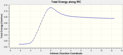  Figure 31: RMS Gradient Graph for IRC Optimisations of the Cycloaddition transition State

The reaction coordinate follows the expected pathway from reactants, over a transition state (via an activation energy barrier) and downhill to the energetically favorable cylocaddition product. This energy barrier will be investigated in the next section;

Activation Energy

The activation energies of the prototype reaction were calculated at 298.15 K and the results are displayed in Table 22. Interestingly the AM1 semi-emprical level of theory provides results which are closer to the cited literature values in comparision to the higher level B3LYP/6-31G*. In order to remain consistent and not introduce a computational error all calulcations were conducted from start to finish using the same basis set optimisation, i.e. structures optimised using the AM1 level of theory were not used as inputs for calculations at a different level of theory at any point during this investigation. The semi-empirical AM1 method is parameterised against experimental data, this may be the main reason why the activation energies produced at this level are more consistent with literature values.

Table 22. Summary of Activation Energy of Prototype Reaction.

Structure	AM1 Sum of Electronic and Thermal Energies at 298.15 K (Ha)	AM1 Activation Energy (kcal mol-1)	B3LYP/6-31G* Sum of Electronic and Thermal Energies at 298.15 K (Ha)	B3LYP/6-31G* Activation Energy (kcal mol-1)	Literature Values (kcal mol-1)
cis-Butadiene	0.138574	24.06999022	-155.906489	16.68671933	27.5
Ethene	0.080252	24.06999022	-78.533191	16.68671933	27.5
DA Transition State	0.259452	24.06999022	-234.413088	16.68671933	27.5

The log files for the AM1-optimised transition state and the B3LYP/6-31G*-optimisted transition states are linked here & here. This concludes the investigation into the prototype Diels-Alder cycloaddition reaction, the next section will investigate a more complex example using many of the computational methods previously employed.

Regioselectivity of Maleic Anhydride + Cyclohexadiene Diels-Alder Cycloadditon

The final part of this computational investigation involves studying the he reaction of maleic anhydride with cyclohexa-1,3-diene to form bicyclo[2.2.2]oct-5-ene-2,3-dicarboxylic anhydride. This reaction is also a thermally allowed suprafacial process obeying the Woodward-Hoffmann rules. The same general methods used above will be employed to study the regioselectivity of this cycloaddition reaction, with respect to the preference via an endo/exo transition state.

Literature states that conducting this reaction under kinetic control (i.e low temperatures and short reaction times) would result in the endo- product being preferentially formed. However, if you increase the temperature of the reaction vessel, and leave the reaction for a longer period of time, the equilibrium shifts to favour the thermodynamic, exo- product. The endo- product is considered to be the kinetic product, which is kinetically favoured due to the stablising secondary orbital interactions present in the transition state, thereby lowering the energy of the transition state relative that of the exo- form. However, it is known that the exo- product is of a lower total energy than the endo- product, due to the larger degree of steric strain present within the endo product.

A reaction scheme depicting these two reactive pathways is shown below, also included is the presence of the destabilising steric hindrance present in the endo-product:

Figure 32: Mechanism of the Diels-Alder Reaction between Maleic Anhydride and Cyclohexadiene

The aim of this final part of the module is to model both the endo- and exo- transition states for the reaction of Maleic Anhydride with Cyclohexadiene, and attempt to rationalise the kinetic preference for the endo- product over the exo- product.

Optimising the Reactants and Products

As with the previous cycloaddition reaction, initially the reactants need to be modeled and optimised before performing any transition state analysis. The reactants were drawn in GaussView 5.0 and optimised to a minimum using the both the semi-empirical AM1 method and the DFT-B3LYP/6-31G* method. The table below summaries the results of these optimisations:

Table 23: Summary of Total Energies and RMS Gradients for the Reactants

Reactant	Structure	Total Energy/Ha	RMS Gradient
Maleic Anhydride (AM1) (log file)		-0.12182418	0.00003683
Cyclohexadiene (AM1) (log file)		0.02771129	0.00000562
Maleic Anhydride (DFT) (log file)		-379.28954412	0.00011730
Cyclohexadiene (DFT) (log file)		-233.41891074	0.00003536

Generating Transition States

The frozen co-ordinate method was again employed to determine the structure of the transition state. The AM1-optimised structures of both reactant molecules were arranged in such a way as to resemble the structure of the expected product molecule for both the exo- and endo- transition states, this was also subsequently performed using the DFT-B3LYP/6-31G* optimised reactants. Similarly to the previous cycloaddition investigation the interatomic distance between the two sets of terminal interacting carbons was frozen to 2.2Å. A semi-empirical AM1-optimisation was performed on both of the endo/exo structures, the same method was performed with the DFT-optimised structures. The co-ordinates of the resultant structures were then unfrozen and set to calculate a derivative, the molecule was subsequently optimised to a transition state using the normal Hessian method.The results of both levels of optimisation to the transition states are given in the table below:

Table 24: Summary of Total Energies and RMS Gradients for the Transition State (AM1 and DFT optimised)

Transition State	Structure	Total Energy / Ha	RMS Gradient
endo (AM1) (log file)		-0.05150437	0.00002354
endo (DFT) (log file)		-612.75578549	0.00000482
exo (AM1) (log file)		-0.05041814	0.00007031
exo (DFT) (log file)		-612.75829022	0.00001074

From the results above it can be concluded that at both levels of optimisation the the endo- transition state is more stable. This is in agreement with the previous discussion earlier in the sections above. However, this data alone does not provide enough information as to why the endo- transition state is more stable, this will be discussed later on in the MO section of the exercise.

Bond Length Analysis of the Transition States

The table below contains all the relevant bond lengths and interatomic distances for the two transition states of this reaction, optimised at the two different levels of theory. Note that 'orientation' defined as the C-C through space distances between the -(C=O)-O-(C=O)- fragment of the maleic anhydride and the C atoms of the “opposite” -CH2-CH2- for the exo and the “opposite” -CH=CH- for the endo.

Table 25: Summary of Bond Lengths and Interatomic Distances for Diels Alder Transition States (AM1 and DFT/6-31G*)

Transition State	Forming C-C Bond Separation/Å	Cyclohexa-1,3-diene C=C Bond Length/Å	Cyclohexa-1,3-diene C-C Bond Length/Å	Maleic Anhydride C=C Bond Length/Å	Maleic Anhydride C=O Bond Length/Å	Orientation/Å
AM1 Optimised (exo-)	2.17	1.39	1.40	1.41	1.22	2.95
DFT B3LYP/6-31G* Optimised (exo-)	1.56	1.51	1.34	1.54	1.20	2.98
AM1 Optimised (endo-)	2.16	1.39	1.40	1.41	1.22	2.89
DFT B3LYP/6-31G* Optimised (endo-)	1.56	1.51	1.34	1.54	1.20	2.99

Upon comparison of the two DFT-optimised transition states, there does not appear to be much difference between the endo- and the exo- product. The same can be concluded for the two AM1-optimised structures, however a notable difference is observed between the two "orientation" (through space interaction) lengths, which is shorter for endo- structure by 0.06Å when compared to the exo- form. As previously shown above the endo product has a lower energy transition state and thus will be the kinetic product for this reaction, the calculation above shows that the bond-forming distance for the endo form is also shorter, again a reason for the preference of formation of the endo product. In contrast, despite the fact that the exo product is lower in energy due to having less unfavourable repulsive steric interactions, the exo transition state lies higher in energy and it will not be observed in reactions which proceed under kinetic control. Instead the exo product is the thermodynamic product in the case of the reaction between maleic anhydride and cyclohexa-1,3-diene. This observation will be supported later during the MO analysis which introduces an additional degree of stabilisation for the endo product, namely secondary orbital overlap.

Frequency Analysis of the Transition States

Prior to the MO analysis, in order to confirm that that that a transition state was successfully obtained, as opposed to a minimum, a frequency analysis was performed on each individual transition state. The data for both the imaginary frequencies and lowest positive vibrational modes for each transition state (optimised to AM1) is given in the table below:

Table 26: Vibrational Analysis for the Transition States (AM1 only)

Transition State	Imaginary Vibrational Frequency/cm-1	Lowest positive Vibrational Frequency/cm-1
endo (AM1)	-807	63
exo (AM1)	-811	60

The presence of a single negative vibrational mode for each transition state confirms that they have all been successfully optimised to transition structures, as opposed to minima or points of inflection.

An animation of each imaginary frequency is shown below for both transition states, this mode displays vibration along the reactive bond forming path of the transition state, in a concerted synchronous manner. In addition to this an animation of the lowest positive vibrational mode is also shown, which displays rotation of the Cyclohexadiene group in the opposite direction to the rotation of the Maleic Anhydride ring in an asynchronous manner, this is comparable with the lowest positive frequency in the Diels-Alder reaction between cis- Butadiene and Ethene, shown previously.

• 
  Figure 33. Animation of imaginary frequency endo (AM1)
• 
  Figure 34. Animation of lowest positive vibration endo (AM1)
• 
  Figure 35. Animation of imaginary frequency exo (AM1)
• 
  Figure 36. Animation of lowest positive vibration exo(AM1)

Molecular Orbital Analysis of the Transition States

The structures of several MO's for both the exo- and endo- (AM1-optimised) transition states were visualised using GaussView. In addition to simulating the HOMO and the LUMO, the structure of the HOMO-1 and LUMO+1 MO's would also be investigated as well as the HOMO-4, in order to gain a greater insight into origin of the secondary orbital overlap effect which acts to stabilise the overall energy of the endo- transition state with respect to the exo- transition state. This interaction should be present in the HOMO of the endo TS however this is evidently not the case for this simulation. The search for the secondary orbital overlap was conducted by visualising the MO's between the HOMO-4 and LUMO+3, not all of the MO's that were visualsed in GaussView are presented below due to their lack of secondary orbital overlap. The stabilising secondary orbital overlap interaction was only found for the LUMO+1 and LUMO+2 for the endo transition structure. It can clearly be seen below that the p-orbitals of the carbonyl carbon on the maleic anhydride overlap in phase with the p-orbitals of the alkene in the cyclohexadiene molecule, leading to an overall energetically stabilising effect. This stabilsing effect is not present in any MO's for the endo state which agrees with both theory and literature and supports the regioselectivity for the endo product during a Diels-Alder cycloaddition. Although this interaction is not observed within the HOMO this can be explained by two factors, the first is that orbital mixing has not been taken into account (What kind of orbital mixing has not been taken into account? João (talk) 21:27, 16 February 2015 (UTC)) during this simple computational experiments, due to the closeness in energy of the respective FMO's substantial mixing upon combining the two reactants would be expected, this may allow the predicted LUMO+1 and LUMO+2 to be involved in bonding interactions and be subsequently populated with electrons. The second factor to consider is simply computational error, this is a simulation and therefore will be subject to numerous errors, due to the use of a low level basis set this could be why the HOMO of the endo TS does not display the expected secondary orbital overlap.

Table 27: Molecular Orbitals of the Transition State (AM1)

Transition State	HOMO-4	HOMO-1	HOMO	LUMO	LUMO+1	LUMO+2
Endo	Symmetric	Symmetric	Anti Symmetric	Anti Symmetric	Symmetric	Symmetric
Exo	Symmetric	Symmetric	Anti Symmetric	Anti Symmetric	Symmetric	Symmetric

Theory suggests that the secondary orbital effect should be observed in the HOMO of the endo transition structure. However on further examination of the orbitals this is not the case, there is no observable in-phase overlap between the carbonyl-based orbitals and the orbitals of the C=C double bond on the cyclohexadiene fragment. However upon inspection that can be seen that this secondary orbtial overlap is present for the endo structure in both the LUMO+1 and the LUMO+2, both of these stabilising overlaps of in phase orbitals is not present in the corresponding MO's for the exo structure. Although the calculation is not perfect, it may also be suggested that this apparent secondary orbital overlap simply does not occur, the LUMO+2 orbitals do not contribute to bonding and can therefore be disregarded, all bonding orbitals (HOMO and lower) show no sign of the supposed secondary orbital overlap, for this specific computational calculation.

IRC Analysis of the Transition States

Similarly to the previous investigation an IRC analysis of the transition states can yield information regarding the expected stability of the products of the cycloaddition reaction. Literature suggests that the exo-product is the thermodynamic product and thus will be the lowest energy product, this was confirmed by the AM1-optimised IRC analysis which was conducted using 50 steps, in both directions and calculating the force constant at every step, finally a standard optimisation of the final step of the IRC yielded the resultant energies for the endo and exo products, which are compared in the table below:

Table 28. Comparison of Transition Structures following Semi-Empirical AM1 IRC.

Structure	Total Energy following AM1 optimisation (Ha)	RMS Gradient	Total Energy vs. IRC	RMS Gradient vs IRC
Endo	-0.159990929	0.00002578
Exo	-0.16017060	0.00003895

It was observed that the exo product was indeed lower in energy by 0.1128 kcal mol^-1. Although this difference is very small it is supported by the literature and shows the ability to elucidate yet another feature of the PES for this reaction. The exo product lies lower in energy on the PES relative to the endo product, this supports the statement above that whislt the kinetic product of this reaction is the endo product, the thermodynamic product is the less sterically hindered exo form.

Activation Energy Investigation

A further investigation into the activation energy for the Diels-Alder reaction between maleic anhydride and cyclohexa-1,3-diene should provide us with evidence for which product endo/exo is thermodynamically favoured. Calculations were conducted at both the AM1 and B3LYP/6-31G* levels of theory and the resultant energy values are compared to that of the literature.

Table 29. Summary of Activation Energies for Endo and Exo Transition States.

Structure	AM1 Sum of Electronic and Thermal Energies at 298.15 K (Ha)	Activation Energy (kcal mol-1)	B3LYP/6-31G* Sum of Electronic and Thermal Energies at 298.15 K	Activation Energy (kcal mol-1)	Literature Activation Energy (kcal mol-1)
Maleic Anhydride	-0.058192	-	-379.228468	-	11.4
1,3-cyclohexadiene	0.157726	-	-233.290922	-	11.4
Endo	0.143679	27.70138481	-612.559977	25.9092191	11.4
Exo	0.144886	28.45878817	-612.562604	27.11717393	11.4

The first observation is that the B3LYP/6-31G* calculations yield results which are slightly closer to the literature values, this would be expected when using the more accurate basis set. The key observation to be pulled from these results however, is that in using both optimisation methods the activation energy for the endo transition state is lower than that of the exo form. This is in perfect agreement with literature which states that the kinetic product, the product formed fastest via the lowest energy barrier transition state is the endo form.

AM1 Method Neglected Factors

To conclude this investigation it should be noted that some factors have been neglected during these calculations; due to the inherent approximations from both the method and basis set chosen. "The first step in reducing the computational problem is to consider only the valence electrons explicitly; the core electrons are accounted for by reducing the nuclear charge or introducing functions to model the combined repulsion due to the nuclei and core electrons. Furthermore, only a minimum basis set (the minimum number of functions necessary for accommodating the electrons in the neutral atom) is used for the valence electrons."^[1] In addition to this "the central assumption of semi-empirical methods is the Zero Differential Overlap (ZDO) approximation, which neglects all products of basis functions that depend on the same electron coordinates when located on different atoms."^[1]

Although the AM1 semi-empirical method allows for relatively fast computational analysis to be conducted to a good level of accuracy it should be noted that this level of theory does suffer from some drawbacks. Known limitations of the AM1 method include:

• predicts hydrogen bond strengths approximately correctly (but often with the wrong geometry)
• hypervalent molecule calulations improved over MNDO method, but still with significant errors
• alkyl groups systematically predicted too stable by approximatley 2 kcal mol^-1 per CH₂ group
• nitro groups too unstable
• peroxide bonds too short
• known to underestimate the rotational barriers for bonds which possess some double bond character

In addition to the list above, Van der Waals interactions are often poorly predicted. It is entirely possible that the absence of the stabilising secondary orbital overlap interaction in the HOMO of the endo transition state is due to one or more of these limitations listed above. Therefore a more accurate analysis of this secondary orbital overlap may require the use of a higher level basis set. However, as demonstrated in the calculations above the semi empirical AM1 method is sufficient in producing results which both agree with the expected theory and give energy values close to those reported in the literature. As with all computational calculations the ability to perform a calculation is no guarantee that the results can be trusted, therefore careful calibration and theoretical rationale should be employed during any computational discussion.

Conclusion

The computational methods employed during this investigation have shown to be successful for modelling the transition states for three separate pericyclic reactions. This highlights a huge advantage of computational chemistry as transition states are known the to posses incredibly short lifetimes, of the order of femtosconds, rendering them impossible to view using conventional spectroscopic techniques. A range of levels of theory were implemented throughout the investigation with each basis set often producing different results, due to the nature of each methods level of approximation. In general the B3LYP/6-31G* level of theory proved to be the most accurate at reproducing results, e.g. activation energies, in agreement with literature values. The optimised transition structures were confirmed via frequency analysis, and were characterised by the presence a single imaginary frequency in the case of a transition structure, as opposed to purely positive vibrations indicative of a minimum along the PES. The resultant imaginary frequency was animated in order to further confirm that the optimised structure found did indeed correspond to the desired transition state. Another advantage of computational chemistry is the ability to visualise the molecular orbitals involved during a reaction, however this was found to be problematic for the the reaction of Maleic Anhydride with Cyclohexadiene, where the expected secondary orbital overlap was not present in the kinetically favoured endoo- transition state. This exemplifies one of the few drawbacks of using simple computational methods, a much more time consuming and advanced basis set would need to be employed to account for both orbital mixing and neglect the approximations of both the AM1 and B3LYP/6-31G* levels of theory. Whilst these low levels of theory have shown to be extremely useful in estimating a range of chemical data consistent with literature values, future work may involve the use of both a higher level basis set and the examination of a wider range of diene and dineophile compounds in order to gain further insight into both the advantages and disadvantages of the mthods employed during this investigation.

References

- ↑ F. Jensen, Introduction to Computational Chemistry, Wiley, Chichester, United Kingdom, 2nd edn., 2007.
- ↑ M. J. Bearpark, A. Simperler, ' Calculating Molecular Geometries', QM3 Quantum Mechanics 3/Core 3rd Year Computational Chemistry Laboratory, Imperial College London, 2014.
- ↑ M. Dewar, Chem. Phys. Lett., 1987, 141, pp.521-524
- ↑ Maluendes et al., J. Chem. Phys., 1990, 93, pp. 5902-5911
- ↑ H. Rzepa, 2nd Year Conformational Analysis Course, 2013, p. 'Alkanes', http://www.ch.ic.ac.uk/local/organic/conf/
- ↑ B. G. Rocque, J. M. Gonzales, H. F. Schaeffer III, Mol. Phys., 100(4), p441-446, 2002.
- ↑ K. N. Hod, S. M. Gustafson, & K. A. Black; J. Am. Chem. Soc., Vol. 114, No. 22, 1992
- ↑ L. S. Bartell1 & R. A. Bonham1; J. Chem. Phys.; 1959; 31; 400. DOI:10.1063/1.1730366
- ↑ Hedberg & Schomaker; J. Am. Chem. Soc.; 1951; 73; 1486.
- ↑ R. S. Rowland, R. Taylor, J. Phys. Chem., 1996, 100(18), 7384-7391.
- ↑ R. B. Woodward & Roald Hoffmann; J. Am. Chem. Soc., Vol. 87, No. 2, 395, 1965 DOI:10.1021/ja01080a054
- ↑ R. B. Woodward & Roald Hoffmann;Selection Rules for Concerted Cycloaddition Reactions; J. Am. Chem. Soc., Vol. 87, No. 9, 2046, 1965 DOI:10.1021/ja01087a034
- ↑ Sauer, J. and Sustmann, R. , Mechanistic Aspects of Diels-Alder Reactions: A Critical Survey. Angew. Chem. Int. Ed. Engl., 19: 779–807, 1980 DOI:10.1002/anie.198007791
- ↑ R. Woodward, R. Hoffmann, J. Am Chem. Soc., 87, 1965, pp. 4388-4389
- ↑ Charles A. Eckert and R. A. Grieger; Mechanistic evidence for the Diels-Alder reaction from high-pressure kinetics; J.Am. Chem. Soc., Vol. 92, No. 24, p7149-7153, 1970