Rep:Mod:AliCMPyear3

Investigation into the Ising Model via Computer Simulation

by Aleksei Zaboronsky. CIDː 01064961.

Introduction

This practical looks at using object-oriented programming to investigate the Ising Model, a physical model used to investigate the behaviour of ferromagnets. This is the second such project completed as part of CMP and makes use of Python as a multi-paradigm programming language which can support object-oriented programming in combination with procedural programming. One of the foremost advantages of object-oriented over procedural programming is that it enables the creation of modules. This allows objects to be created which inherit many already existing features of other objects, making object-oriented code easier to modify. A second key advantage of object-oriented programming is that of abstraction. Through data abstraction, programs are made more optimal, because all data apart from specific, relevant data relating to the object being called is hidden. This increases efficiency and allows the program to perform faster.

The project introduces the use of new functions, such as np.roll(), and begins to assess efficiency of code. It explores modelling different sized lattices for the Ising model and extends to an investigation into how the lattice size affects the Curie Temperature of the lattice system. This is done by finding energy variation over temperature and then, from this value, finding the heat capacity against temperature. This process involved the use of simulations of lattices of different sizes and then polyfitting of curves to find maximum heat capacities. The final value of Curie Temperature for an infinite lattice found was 2.271 K, which is in agreement with the literature value of 2.269 K . Since this practical is primarily a coding exercise, the full, annotated code for the IsingModel.py file is presented in the Code and Conclusion section.

Noteː All of the questions in this report are copied from the lab script for this project, which is referenced as for the entire report.

Introduction to the Ising Model

Task 1

Show that the lowest possible energy for the Ising model is $$\begin{gathered} E \\ = \\ -DNJ \end{gathered}$$, where $D$ is the number of dimensions and $N$ is the total number of spins. What is the multiplicity of this state? Calculate its entropy.

The total degrees of freedom (number of nearest neighbours) any one atom has is twice the dimension it is in (i.eː in 2D, an atom has four adjacent atoms, in 3D it has six etc.). Therefore, for N atoms in a system of D dimensions, there are 2ND interactions. Since the system is at the lowest possible energy, all of the atoms have parallel spins; they are either all up or down. Due to this, their spins can be excluded from the energy term, since it is always the case that

$s_i{s}_j=1$

Therefore, the equation for interaction energy

$$\begin{gathered} E=-\frac{1}{2}J\sum _i^N\sum _{j \\ \in \\ \mathrm{n}\mathrm{e}\mathrm{i}\mathrm{g}\mathrm{h}\mathrm{b}\mathrm{o}\mathrm{u}\mathrm{r}\mathrm{s}\left(i\right)}{s}_i{s}_j \end{gathered}$$

becomes

 $E=-\frac{1}{2}J2ND=-DNJ$

where J is the interaction energy.

The multiplicity of this state is 2, since it can either be all spin up or all spin down. Therefore, the entropy of this system is

 $S=k_{B}ln\mathrm{\Omega }=k_{B}ln2$

Task 2

Imagine that the system is in the lowest energy configuration. To move to a different state, one of the spins must spontaneously change direction ("flip"). What is the change in energy if this happens ($$\begin{gathered} D=3, \\ N=1000 \end{gathered}$$)? How much entropy does the system gain by doing so?

At lowest energy state, energy is - 3000J. If one spins is flipped, the energy change is + 12J.

Entropy gainː

$S=k_{B}ln\mathrm{\Omega }=k_{B}ln2000-k_{B}ln2=k_{B}ln1000$

Task 3

Calculate the magnetisation of the 1D and 2D lattices in figure 1. What magnetisation would you expect to observe for an Ising lattice with $$\begin{gathered} D=3, \\ N=1000 \end{gathered}$$ at absolute zero?

The magnetisation for both the 1D and the 2D lattices in figure 1 is + 1; for the 1D lattice there are three spin up atoms, and two spin down atoms, whilst in the 2D lattice there are 13 spin up and 12 spin down.

For the 3D lattice at absolute zero, the system would take the lowest energy configuration, and hence all of the atoms would have parallel spins, whether this was pointing up or down. Therefore, the magnetisation of the 1000 N system at absolute zero would be ± 1000.

Calculating the Energy and Magnetisation

Task 1

Complete the functions energy() and magnetisation(), which should return the energy of the lattice and the total magnetisation, respectively. In the energy() function you may assume that $J=1.0$ at all times (in fact, we are working in reduced units in which $J=k_B$, but there will be more information about this in later sections). Do not worry about the efficiency of the code at the moment — we will address the speed in a later part of the experiment.

The code for this task is seen in figure 1. The energy() function is written as a nested for loop which has two variables i and j to run through the randomly generated lattice rows and columns respectively. It takes each atom and calculates its interactions with all four adjacent atoms. Since the system is taken to have periodic boundary conditions, the interactions for atoms on the edge of the lattice with those on the other side of the lattice are calculated using the Python modulus function, which is called via a % symbol. The factor of ½ is present in order to take into account the nested loop factoring each interaction twice. Since the energy is summed during the loop, it is initially set to zero when the energy() function is called.

Whilst the magnetisation() function could also be written using a for loop, it is more optimal to use the numpy.sum() function, which simply sums the values of every element in an array, in this case the lattice.

The lattice is generated elsewhere in the code (see figure 2), and is called using the syntax self.lattice.

Figure 1ː Initial code for the energy() and magnetisation() functions.

Figure 2ː Code which initialises the lattice, filling it with either plus or minus 1.

Task 2

Run the ILcheck.py script from the IPython Qt console using the command

%run ILcheck.py

The displayed window has a series of control buttons in the bottom left, one of which will allow you to export the figure as a PNG image. Save an image of the ILcheck.py output, and include it in your report.

Upon completion of the energy() and magnetisation() functions, the ILcheck.py program was run to confirm that they were working correctly. Figure 3 below shows the PNG image saved from one of these checks. It confirms that the functions are outputting the correct values, since they are the same as the expected values.

Figure 3ː Image outputted by running of the ILcheck.py file, which confirms that the energy() and magnetisation() functions work correctly.

Introduction to the Monte Carlo Simulation

Task 1

How many configurations are available to a system with 100 spins? To evaluate these expressions, we have to calculate the energy and magnetisation for each of these configurations, then perform the sum. Let's be very, very, generous, and say that we can analyse $1\times 10^9$ configurations per second with our computer. How long will it take to evaluate a single value of ${⟨M⟩}_T$?

Total configurations available is 2^N, so for a system with 100 spins, that is 2¹⁰⁰. Therefore, it would takeː

2¹⁰⁰ / 10⁹ = 1.27 x 10²¹ seconds

1.27 x 10²¹ / 3600 = 3.52 x 10¹⁷ hours

3.52 x 10¹⁷ / 24 = 1.47 x 10¹⁶ days

1.47 x 10¹⁶ / 365 = 4.02 x 10¹³ years

This length of time is longer than the age of the universe. Hence, we need to look for other alternatives...

Task 2

Implement a single cycle of the above algorithm in the montecarlocycle(T) function. This function should return the energy of your lattice and the magnetisation at the end of the cycle. You may assume that the energy returned by your energy() function is in units of $k_B$! Complete the statistics() function. This should return the following quantities whenever it is called: $<E>,<E^2>,<M>,<M^2>$, and the number of Monte Carlo steps that have elapsed.

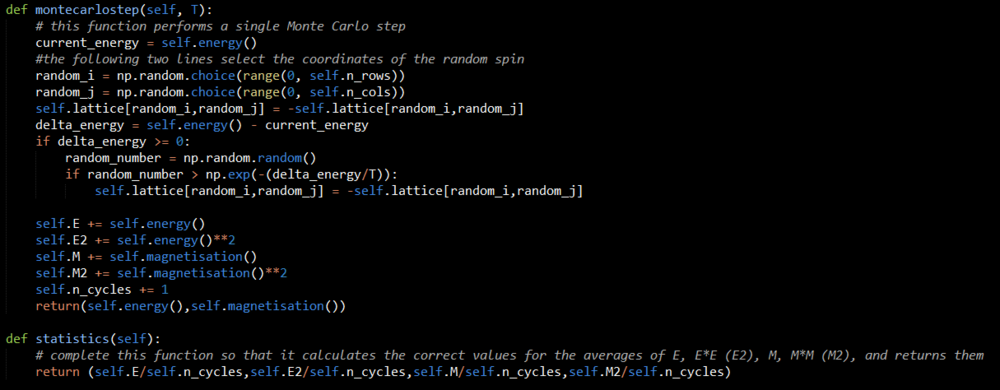
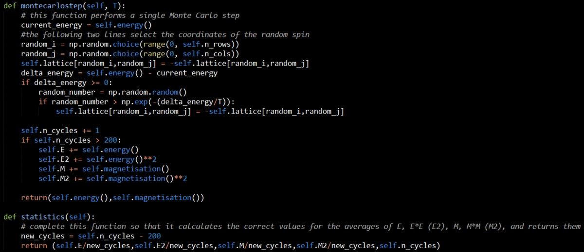
Figure 4 shows the code written to implement a Monte Carlo Step and also the statistics() function. The montecarlostep(T) function takes the temperature in Kelvin as an input. It sets the energy to the current energy by calling the energy() function discussed in the previous section. It then selects a random atom in the lattice and flips its spin. It then calculates the energy difference between the initial state and the new state (with the newly flipped atom). If the new state has a lower energy than the previous one, the system is kept in this arrangement, and a Monte Carlo Step has been completed. If, however, the new state is of higher energy, a random number is generated. This number is then compared to the probability of a transition from one state to another occurring. If the random number is less than or equal to this value, the new configuration is retained.This step determines whether the higher energy state is kept or if the system reverts to its previous, lower energy state. At this point in the montecarlostep(T) function, the running variables tracking the energy, magnetisation, those two quantities squared and the number of Monte Carlo Steps are updated. The function outputs the energy and magnetisation of the lattice at the time it is called upon. The statistics() function takes the running totals created in the montecarlostep(T) function and calculates their average values by dividing through by the number of cycles run. It returns these values. The iteration of this code shown in figure 4 only returns four variables. However, the code was then edited to return five outputs, the final one being the number of cycles run. This is seen in the overall code discussion in the final section of this report.

Figure 4ː Code written to implement a single Monte Carlo step and output the energy, magnetisation, and those values squared upon the calling of the statistics() function.

Task 3

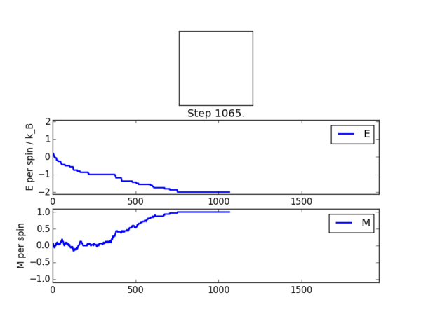
If $T<T_C$, do you expect a spontaneous magnetisation (i.e. do you expect $⟨M⟩\ne 0$)? When the state of the simulation appears to stop changing (when you have reached an equilibrium state), use the controls to export the output to PNG and attach this to your report. You should also include the output from your statistics() function.

Yes, at a temperature below the Curie Temperature, the system would be expected to spontaneously magnetise, as it adopts its lowest energy configuration. Figure 5 shows the PNG image saved from the ILanim.py file run. In this case, the equilibrium state was achieved after apporoximately 750 steps. This can be seen by the energy and magnetisation per spin stabilising and all of the atoms having parallel spins.Figure 6 shows the output from the statistics() function to go along it.

Figure 5ː Saved image taken from running the ILanim.py file, showing the equilibrium state being reached after approximately 750 steps.

Figure 6ː Output from the statistics() function for the run seen in figure 5.

Accelerating the Code

Task 1

Use the script ILtimetrial.py to record how long your current version of IsingLattice.py takes to perform 2000 Monte Carlo steps. This will vary, depending on what else the computer happens to be doing, so perform repeats and report the error in your average!Look at the documentation for the NumPy sum function. You should be able to modify your magnetisation() function so that it uses this to evaluate M. The energy is a little trickier. Familiarise yourself with the NumPy roll and multiply functions, and use these to replace your energy double loop (you will need to call roll and multiply twice!).Use the script ILtimetrial.py to record how long your new version of IsingLattice.py takes to perform 2000 Monte Carlo steps. This will vary, depending on what else the computer happens to be doing, so perform repeats and report the error in your average!

Noteː the three tasks for this section are being reported as one because it seemed more logical to report them and compare results together.

Initially, the ILtimetrial.py file was run, which recorded the time taken for 2000 Monte Carlo steps to be completed. This, and the results (with error) are all recorded in table 1. Before implementing the suggested improvements, another improvement was made to the energy() function, which is seen in figure 7. The change removes the factor of ½ and calculates each interaction between neighbours once instead of doubling it up. It does this by only calculating the interaction with the atom to the right and below the atom in question in the lattice. Since the function runs through the whole lattice, this yields the same result, and is far more efficient. This modification is referred to as optimisation 1 in table 1.

Figure 7ː Initial code optimisation, removing the two time counting of interactions.

Figure 8 shows the code for the energy() function optimised using the numpy.roll() and numpy.multiply() functions. This method removes the need for any for loops and takes advantage of the ability to perform (in this case) matrix multiplication and manipulation. This drastically decreases the run time, as seen in table 1, since the lattice points are all multiplied together simultaneously, not one by one. This modification is referred to as optimisation 2 in table 1. Figure 8 doesn't show the magnetisation() function because it already made use of the numpy.sum() function, as seen in figure 1.

Figure 8ː Second code optimisation, making use of the numpy.roll() function.

Table 1ː Table showing the decreasing run time for performing 2000 Monte Carlo Steps after implementing optimising modifications to the energy() function.

Stage	Mean Time / s	Standard Deviation / s	Standard Error / s
Before optimisation	37.66427881	0.231450138	0.103507648
After first optimisation	8.362681111	0.016213448	0.007250874
After second optimisation	0.526759674	0.007416936	0.003316954

The Effect of Temperature and System Size

Task 1

The script ILfinalframe.py runs for a given number of cycles at a given temperature, then plots a depiction of the final lattice state as well as graphs of the energy and magnetisation as a function of cycle number. This is much quicker than animating every frame! Experiment with different temperature and lattice sizes. How many cycles are typically needed for the system to go from its random starting position to the equilibrium state? Modify your statistics() and montecarlostep() functions so that the first N cycles of the simulation are ignored when calculating the averages. You should state in your report what period you chose to ignore, and include graphs from ILfinalframe.py to illustrate your motivation in choosing this figure.

After running many tests, it becomes apparent that the number of cycles which can be ignored varies drastically as the lattice size and temperature of the system are varied. This can be seen clearly by looking at figures 9 and 10; whilst in figure 9, equilibrium is reached almost instantly (after approximately 150 steps), in figure 10, the energy is still decreasing by the time 100,000 steps have passed. This vast difference is due to differing lattice sizes. Figure 9 is for a 6 by 6 lattice at 1 K and figure 10 is for a 32 by 32 lattice at 1 K.

Figure 9ː Energy per spin and magnetisation per spin for a 6 by 6 lattice at 1 K.

Figure 10ː Energy per spin and magnetisation per spin for a 32 by 32 lattice at 1 K.

Figure 11 below shows the edited code for the montecarlostep(T) and statistics() functions to ignore a set number of steps. The inserted example in figure 11 ignores 200 steps, which is the number chosen specifically for a 6 by 6 system at a temperature of 1 K. Figure 9 shows the graph at these conditions, which illustrates why the number 200 was chosen, since after approximately 150 steps equilibrium has been reached. This means that the program only takes readings after this value, hence the average at the end is more accurate. The code edit works by inputting this chosen number. Then, the running counters for total energy, magnetisation and those quantities squared are only added up after this number has been passed. The statistics() function then takes this number away from the number of steps at that point and divides through by this edited value to provide a fair mean for the steps taken after the "ignore-value" number has been passed.

Figure 11ː Edited code for the montecarlostep(T) and statistics() functions in order to ignore a set number of steps. In this example, the number chosen to ignore is 200.

To consider the effect of temperature, an 8 by 8 lattice was tested at 1, 2, 3, 5, 50 and 100 K. Table 2 below shows the graphs for these runs. As can be seen, all of these runs reach equilibrium well within the 150,000 steps recorded. However, the equilibrium state looks wildly different for the systems at 1 and 2 K and those at higher temperatures. This is to say that, at 1 and 2 K, the system fully magnetises, with all of the atoms adopting the same spin (either all up or all down). However, for the systems at a temperature of 3 K or higher, the equilibrium state does not result in all parallel spins, but rather the spins seem to be totally random. This suggests that the Curie Temperature for an 8 by 8 lattice lies between 2 and 3 K. Therefore, below this temperature, the system adopts the most energetically favourable alignment (all the spins being parallel). However, above this temperature the system becomes entropy dominant and hence the equilibrium state of the system is all of the spins randomly being either up or down. This is because this maximises the multiplicity, and hence entropy, of the system.

Table 2ː Table showing the effect of temperature on time for system to reach equilibrium for an 8 by 8 lattice.

Graph	Temperature / K
	1
	2
	3
	5
	50
	100

Task 2

Use ILtemperaturerange.py to plot the average energy and magnetisation for each temperature, with error bars, for an $8\times 8$ lattice. Use your intuition and results from the script ILfinalframe.py to estimate how many cycles each simulation should be. The temperature range 0.25 to 5.0 is sufficient. Use as many temperature points as you feel necessary to illustrate the trend, but do not use a temperature spacing larger than 0.5. The NumPy function savetxt() stores your array of output data on disk — you will need it later. Save the file as 8x8.dat so that you know which lattice size it came from.Repeat this task for the following lattice sizes: 2x2, 4x4, 16x16, 32x32. Make sure that you name each datafile that your produce after the corresponding lattice size! Write a Python script to make a plot showing the energy per spin versus temperature for each of your lattice sizes. Hint: the NumPy loadtxt function is the reverse of the savetxt function, and can be used to read your previously saved files into the script. As before, use the plot controls to save your a PNG image of your plot and attach this to the report. How big a lattice do you think is big enough to capture the long range fluctuations?

Noteː the sections looking at effects of temperature and system size have been combined in order to better convey the results whilst altering both variables.

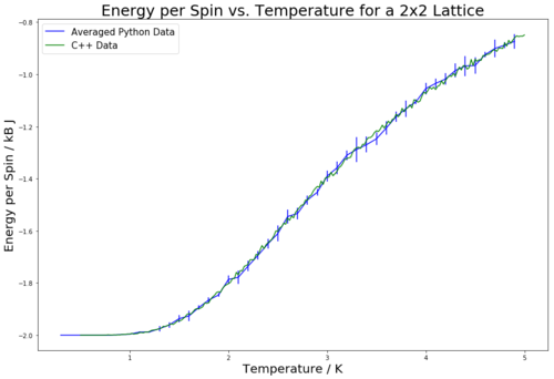
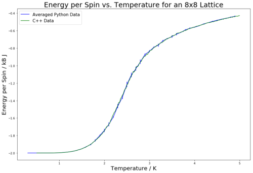
Table 3 shows the obtained graphs for energy vs temperature and magnetisation vs temperature for varying lattice sizes. The data is plotted against the provided C++ data to show the comparison of values. Each run was performed five times, and the graphs plot the average value of energy/magnetisation for each temperature step. The error bars are plotted by use of the standard deviation calculated from the five repeats. For all of the lattice sizes except 32 by 32, the temperature was varied between 0.3 and 5.0 K with a 0.1 K step size. For the 32 by 32 lattice, it was varied from 0.25 to 5.0 K with a 0.25 K step size. This is due to the 32 by 32 lattice requiring a larger number of steps to collect accurate data. Hence, to save time, the step size was increased from 0.1 to 0.25 K for these runs. Table 3 contains the number of steps run and ignored at the start of the run for each lattice size. The way these numbers were determined was by running the ILfinalframe.py program for the given lattice sizes at 0.3, 1, 2.5 and 5 K and then determining from the outputted results how many steps would be needed for a good run and how many from the start needed to be discarded to ensure a good calculation of energy/magnetisation. The data obtained for energy matched the provided C++ data very closely, and had little error. The magnetisation also matched the provided data; while it shows large fluctuations and error at the lower temperatures, it stabilises to closely match the provided data as the temperature increases above 3 K. It can be seen that the error is lower for the 32 by 32 lattice than for the other lattice sizes. This is to be expected, since there are more atoms, and hence a higher level of averaging. Due to this, there are still errors, however their magnitude is diminished.

Table 3ː Table showing the effect of temperature and system size on the energy per spin and magnetisation per spin of atoms in lattices of varying sizes.

Energy vs. Temperature Graph	Magnetisation vs. Temperature Graph	Total Steps	Ignored Steps
		10,000	1,000
		10,000	1,000
		100,000	10,000
		50,000	10,000
		200,000	100,000

By looking at the magnetisation vs. temperature curves in table 3, it can be seen that the larger the lattice size, the lower the long range fluctuations occurring through the system. This can be seen from the flatter tails for the 32 by 32 and 18 by 16 lattices as compared to the 4 by 4 and 2 by 2 lattices. It would be expected that, as the size of a lattice tends to infinity, the fluctuations would be minimised even more so, resulting in a smoother transition region curve.

Determining the Heat Capacity

Task 1

By definition,

$C=\frac{\partial ⟨E⟩}{\partial T}$

From this, show that

$C=\frac{\mathrm{V}\mathrm{a}\mathrm{r}[E]}{k_B{T}^2}$

(Where $\mathrm{V}\mathrm{a}\mathrm{r}[E]$ is the variance in $E$.)

Answerː

Taking the partition function

$Z=\sum _n{e}^{-\beta E_n}$,

the canonical ensemble average energy

$⟨E⟩=\frac{\sum _n{E}_n{e}^{-\beta E_n}}{\sum _n{e}^{-\beta E_n}}$ 

can be expressed as

$⟨E⟩=-\frac{1}{Z}\frac{\partial Z}{\partial \beta }=-\frac{\partial logZ}{\partial \beta }$

The variance shows spread of energies about the mean (probability distribution fluctuations) and is mathematically expressed asː

$Var[E]=\mathrm{\Delta }{E}^2=⟨(E-⟨E⟩{)}^2⟩=⟨E^2⟩-{⟨E⟩}^2$

From this equation, it is clear that, if the mean values of both the energy and the energy squared are known, the variance can be calculated. The variance expression can also be written in terms of the partition function Zː

$\mathrm{\Delta }{E}^2=\frac{{\partial }^2}{\partial {\beta }^2}logZ=-\frac{\partial ⟨E⟩}{\partial \beta }$

Now this can be linked to another expression for fluctuations; the heat capacity definition in the canonical ensemble (energy is not fixed)ː

$C_v=\frac{\partial ⟨E⟩}{\partial T}{|}_v$

Noting that

$\beta =\frac{1}{k_{b}T}$,

combining the previous two equations givesː

$C=\frac{\mathrm{V}\mathrm{a}\mathrm{r}[E]}{k_B{T}^2}$

Task 2

Write a Python script to make a plot showing the heat capacity versus temperature for each of your lattice sizes from the previous section. You may need to do some research to recall the connection between the variance of a variable, $\mathrm{V}\mathrm{a}\mathrm{r}[X]$, the mean of its square $⟨X^2⟩$, and its squared mean ${⟨X⟩}^2$. You may find that the data around the peak is very noisy — this is normal, and is a result of being in the critical region. As before, use the plot controls to save your a PNG image of your plot and attach this to the report.

Figures 12 to 16 show the heat capacity plotted against the temperature for the required lattice sizes. The heat capacity was found using the equation containing variance derived in the previous section. This was done for all five energy runs for each lattice size, hence five heat capacity values were found for each lattice size. This allowed the mean and standard deviation to be found. The mean is plotted in these graphs, with the standard deviation once again being used to form error bars. All of the data is plotted against the C++ data provided for comparison. Legends on the graphs denote which data is which. The collected data matches the provided data quite closely. As expected, the data has higher fluctuations around the peak. This is a result of it being the critical region. This can be clearly seen on the graphs by the error bars increasing in size at the peak and tailing off almost completely once the peak has been passed. This is particularly noticeable for the 16 by 16 and 32 by 32 lattices (figures 15 and 16).

Figure 12ː Heat capacity vs. temperature for a 2 by 2 lattice.

Figure 13ː Heat capacity vs. temperature for a 4 by 4 lattice.

Figure 14ː Heat capacity vs. temperature for an 8 by 8 lattice.

Figure 15ː Heat capacity vs. temperature for a 16 by 16 lattice.

Figure 16ː Heat capacity vs. temperature for a 32 by 32 lattice.

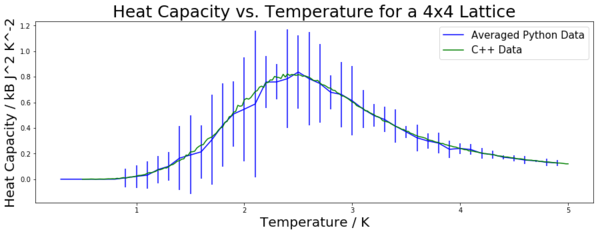
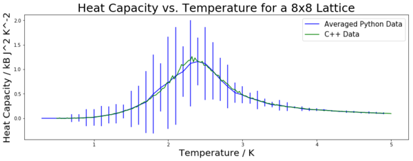
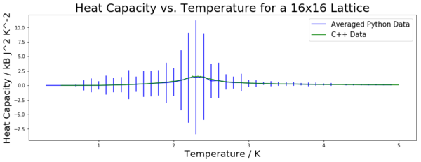
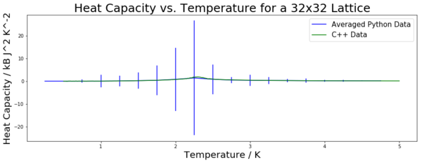
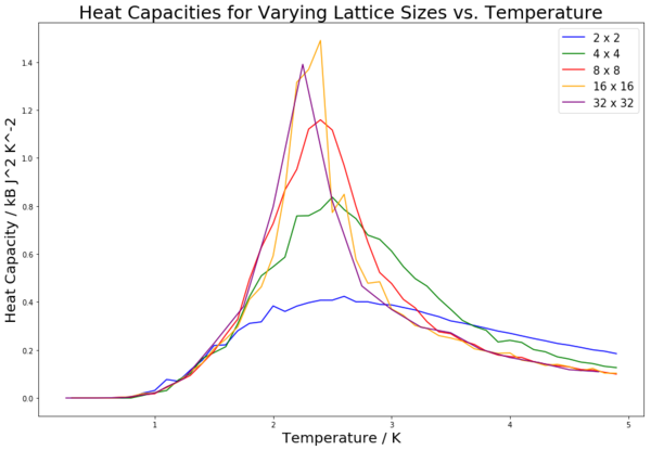
Figure 19 is a compilation of all of the heat capacity curves from figures 12 to 16 on one graph. The plots are still the mean values, but the error bars are not shown in order to better compare the curves. It can be seen that, as lattice size increases, the peak section becomes increasingly sharply peaked. This is to be expected, and in fact if the system was increased to an infinite system, the heat capacity would be expected to diverge at the maximum point of the peak (which occurs at the Curie Temperature).

Figure 17ː Heat capacity vs. temperature for varying lattice sizes.

Locating the Curie Temperature

Task 1

A C++ program has been used to run some much longer simulation than would be possible on the college computers in Python. For each lattice size, plot the C++ data against your data. For one lattice size, save a PNG of this comparison and add it to your report — add a legend to the graph to label which is which.

This has been done, and can be seen in figures 12 to 16.

Task 2

Write a script to read the data from a particular file, and plot C vs T, as well as a fitted polynomial. Try changing the degree of the polynomial to improve the fit — in general, it might be difficult to get a good fit! Attach a PNG of an example fit to your report.

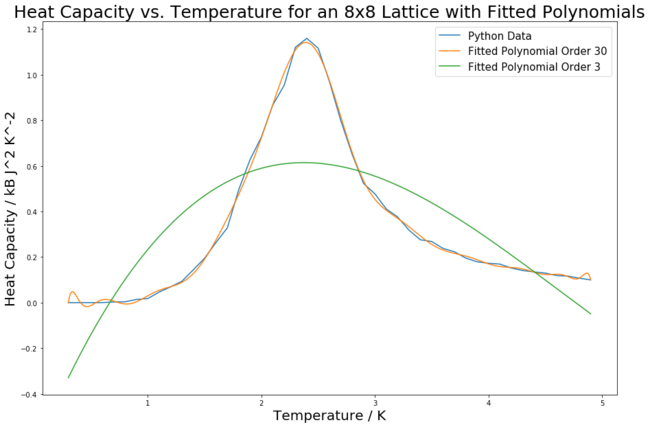
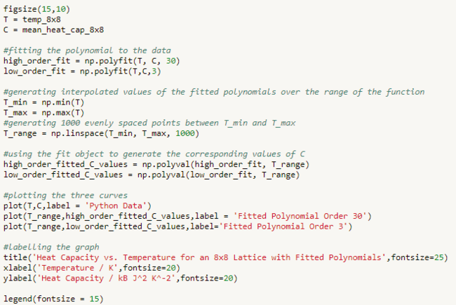
Figure 18 shows the heat capacity curve for an 8 by 8 lattice collected from the python simulations. As before, the curve is plotted using mean values, and the error bars have been removed to allow a more clear view of the fit. Experimentation with the polynomial degree led to a remarkably good fit being obtained for an order 30 polynomial. This is in contrast to a third order polynomial, which resulted in an unsatisfactory fit. Both order polynomials are shown in figure 18 to provide comparison. The fitted curves were obtained using the numpy.polyfit() and numpy.polyval() functions. The annotated code for this is shown in figure 19.

Figure 18ː Heat capacity vs. temperature for an 8 by 8 lattice with fitted polynomials of varying order.

Figure 19ː Code used to generate the graph in figure 18.

Task 3

Modify your script from the previous section. You should still plot the whole temperature range, but fit the polynomial only to the peak of the heat capacity! You should find it easier to get a good fit when restricted to this region.

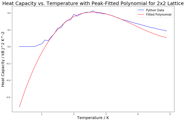
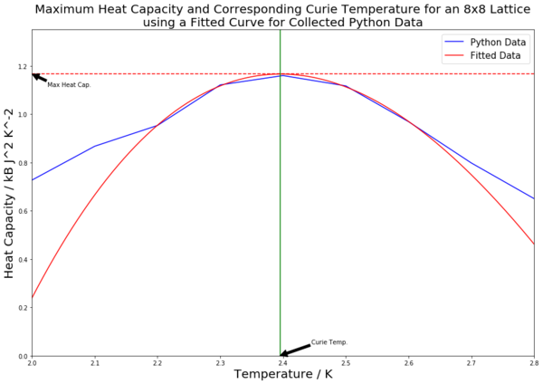
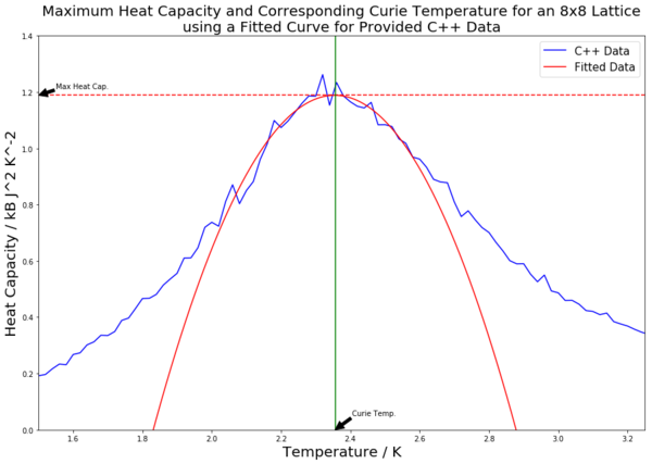
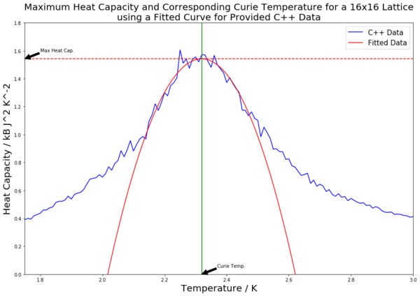
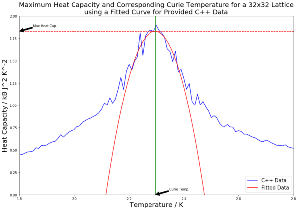
The code was edited to implement a fitted polynomial to be fitted specifically on the peak. Figure 20 shows an example of one of these plots. It is clear to see that the fitted polynomial fits very well on the peak of the heat capacity curve, but then drops away from the rest of the curve. This change to the code meant that lower order polynomials could be used to obtain good fits for the peak. For example, the fitted polynomial used for the graph in figure 20 is only a third order polynomial, yet it fits the peak very closely.

Figure 20ː Heat capacity vs. temperature graph with fitted polynomial which is fitted only to the peaks of the heat capacity.

Task 4

Find the temperature at which the maximum in C occurs for each datafile that you were given. Make a text file containing two columns: the lattice side length (2,4,8, etc.), and the temperature at which C is a maximum. This is your estimate of $T_C$ for that side length. Make a plot that uses the scaling relation given above to determine $T_{C,\mathrm{\infty }}$. By doing a little research online, you should be able to find the theoretical exact Curie temperature for the infinite 2D Ising lattice. How does your value compare to this? Are you surprised by how good/bad the agreement is? Attach a PNG of this final graph to your report, and discuss briefly what you think the major sources of error are in your estimate.

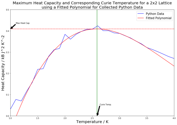
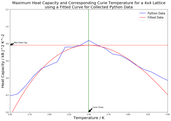
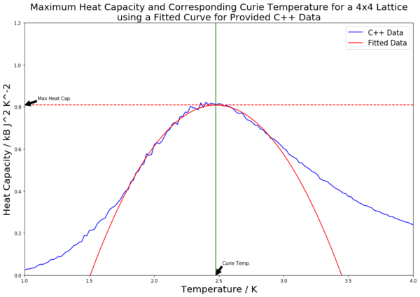
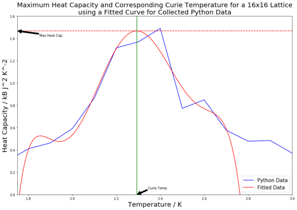
Table 4 contains all of the fitted heat capacity peaks for the varying lattice sizes. As can be seen from the figures in the table, most of the peaks are fitted very closely. The python code was edited so as to record the maximum heat capacity value (from the fitted polynomials). This was done using the numpy.max() function. A horizontal line was then inputted to mark the maximal heat capacity. From this, the corresponding temperature value was found (the Curie Temperature), and a vertical line was inputted to mark this point on the x axis. Both of these points were labelled using the annotate() function. The Curie Temperatures for each graph were saved to an array, which was later used to plot figure 21.

Table 4ː Table showing the fitted peaks for heat capacity for various lattice sizes for both provided C++ data and collected Python data.

Python Data	C++ Data

The scaling relation $T_{C,L}=\frac{A}{L}+T_{C,\mathrm{\infty }}$ can be written as $T_{C,L}=A\frac{1}{L}+T_{C,\mathrm{\infty }}$ to fit the form $y=mx+c$. Therefore, since the constant A is not being considered, plotting the Curie Temperature, which has been found via the fitting polynomials seen in table 4, on the y axis against 1/L (the inverse of the lattice side length) on the x axis should result in a straight line with a y-intercept value equal to the Curie Temperature of an infinite lattice. This has been done for both the collected and provided data, and both lines are plotted in figure 21. The straight lines of best fit were generated using the polyfit() function.

Figure 21ː Plot used to find the Curie Temperature of an infinite lattice.

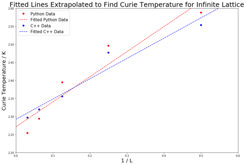
The following Curie Temperatures were found:

C++ data: 2.292 K (3 d.p.)

Python data: 2.271 K (3 d.p.)

A literature source states the theoretical exact Curie Temperature to be 2.269 K (3 d.p) This value is in very good agreement with the 2.271 K value obtained from the collected python data. It is less close, but still near, to the C++ data value of 2.292 K. The level of agreement is not surprising, since all of the data was collected over long, thought-through step numbers and with a small step increment. All runs were repeated and averaged, helping to reduce any error. The maths was calculated correctly and the fits were done specifically to the peaks of the curves. All of this together culminates in a thorough investigation which has produced an accurate final answer, as attested to by the literature.

One of the main sources of error in the experiment is the high level of error for the heat capacity curves. This is particularly clear when looking at figure 16 and the size of the error bars on the peak of the curve. This can be attributed to several factors; firstly, the large fluctuations which occur at that point, which are characteristic of a critical region. Secondly, the error present for energy and energy squared values is increased due to taking those values and squaring the energy when calculating first the variance and then the heat capacity. This spreads the values, increasing the error, and would not occur if heat capacity was being measured directly. From this point, there also arises the error in the polynomial fitting of the curves when calculating the Curie Temperatures for the different lattice sizes. Whilst the fits were worked on to make them as accurate as possible, not all were perfectly fitted. Take, for example, the fitting for the 16 by 16 lattice for the python data. As well as this, in order to make the experiment more time viable, the 32 by 32 lattice runs were calculated with a 0.25 K temperature step size, not 0.1 K as for the other lattice sizes. This larger step size could lead to a more jagged curve and hence miss out on the true maximum value. This would contribute to error and sway the straight line in the final plot in figure 21. Finally, there is the chance that the simulation running did not fully reach equilibrium for some runs, which would increase the likelihood of error.

Code and Conclusion

The following script is the final, annotated code for the IsingLattice.py file.

 
import numpy as np

class IsingLattice:

    E = 0.0
    E2 = 0.0
    M = 0.0
    M2 = 0.0

    n_cycles = 0

    def __init__(self, n_rows, n_cols):
        "Initiate the lattice."
        self.n_rows = n_rows
        self.n_cols = n_cols
        self.lattice = np.random.choice([-1,1], size=(n_rows, n_cols))

    def energy(self):
        "Return the total energy of the current lattice configuration."
        energy = -np.sum(np.multiply(self.lattice,np.roll(self.lattice,-1,axis=0)) + np.multiply(self.lattice,np.roll(self.lattice,-1,axis=1)))
        return energy

    def magnetisation(self):
        "Return the total magnetisation of the current lattice configuration."
        magnetisation = np.sum(self.lattice)
        return magnetisation

    def montecarlostep(self, T):
        # this function performs a single Monte Carlo step
        current_energy = self.energy()
        #the following two lines select the coordinates of the random spin
        random_i = np.random.choice(range(0, self.n_rows))
        random_j = np.random.choice(range(0, self.n_cols))    
        self.lattice[random_i,random_j] = -self.lattice[random_i,random_j] #this flips the randomly chosen spin
        delta_energy = self.energy() - current_energy
        if delta_energy >= 0:
            random_number = np.random.random()
            #compares random number to probability of transition
            if random_number > np.exp(-(delta_energy/T)):
                self.lattice[random_i,random_j] = -self.lattice[random_i,random_j]

        #updates variables
        self.n_cycles += 1
        if self.n_cycles > 100000:
            self.E += self.energy()
            self.E2 += self.energy()**2
            self.M += self.magnetisation()
            self.M2 += self.magnetisation()**2
        
        return(self.energy(),self.magnetisation())

    def statistics(self):
        # complete this function so that it calculates the correct values for the averages of E, E*E (E2), M, M*M (M2), and returns them
        new_cycles = self.n_cycles - 100000
        return (self.E/new_cycles,self.E2/new_cycles,self.M/new_cycles,self.M2/new_cycles,self.n_cycles)

The project was completed successfully, and ended with finding an accurate value of the Curie Temperature for an infinite lattice by finding the intercept on a graph of Curie Temperature vs. 1/Lattice Side Length. Errors were minimised via repeats and included where relevant in the form of standard deviation error bars. Analysis of possible errors is done in the final task of the "Locating the Curie Temperature" section of the report. If the experiment was to be run again, there are several improvements that could be made. One would be relating to the montecarlostep(T) function; when the function was modified to ignore a certain number of initial steps, it was done by hard-wiring in a number via a manual input. A good improvement to make to this would be to write a function such that this number of steps is automatically determined by the function after the energy has been constant for a set number of steps. This would allow the program to work for any lattice size/temperature and would not require user input for the number of steps to be ignored. As well as this, more repeats with a lower temperature step increment, particularly around the heat capacity peak, would allow for a more comprehensive look at the fluctuations at the peak. This would in turn improve the quality of fitting and hopefully yield a more accurate final answer.

As already mentioned in the introduction, a large part of this investigation revolved around the use of object-oriented programming in python. This process has the advantage of higher efficiency than procedural programming due to data abstraction. In this experiment, it was successfully made use of to complete the investigation in a viable time frame.

References

- ↑ 1.0 1.1 Lab Script for this practical, https://wiki.ch.ic.ac.uk/wiki/index.php?title=Third_year_CMP_compulsory_experiment/Introduction_to_the_Ising_model
- ↑ 2.0 2.1 Eltinge, S.L., Numerical Ising Model Simulations on Exactly Solvable and Randomized Lattices, M.I.T., 2015, 1.
- ↑ Tong, D., Statistical Physics, Cambridge University Press, 2012, 20.