
Rep:Mod:Alex Powel Transition States and Reactivity
Introduction
This computational experiment explores the transitions states and reactivity of pericyclic reactions. Initially the [3,3]-sigmatropic rearrangement, namely the Cope rearrangement, will be considered, with the aim of developing the use of optimisation and frequency analysis of a variety of structures using different levels of theory. This was achieved following the use of the laboratory tutorial [1]. The results and discussion arising from the calculations can be found below. Secondly, the Diels Alder cycloaddition was studied in the cases of cis-butadiene and ethene, followed by an investigation into the regioselectivity of reaction between cyclohexa-1,2-diene and maleic anhydride. The computations were carried out using the GaussVeiw 5.0.9 software. It should be noted that in many cases throughout the experiment that the summary file outputted by each computation has been included. This is to allow easy comparisons for those repeating a computation as well as to display the key information, such as the level of theory, job type and energies.
Pericyclic Reactions
The reactions under study are all assumed to pass through a cyclic transition state in a concerted fashion, thus making them pericyclic. Such reactions have been analysed in detail during the years, in particular by Woodward and Hoffmann, who developed their own set of rules for predicting the out come of a pericyclic reaction.[2] These have been simplified to the following form:
Where q and r are both integers and s and a correspond to suprafacial (π/σ system reacts forming bonds on the same face of the orbital) and antarafacial (π/σ system reacts to form bonds on opposite faces) respectively.[2](Note: this is only for thermally controlled reactions; photochemical reactions obey a different rule).

The equation allows frontier molecular orbital analysis of π systems to predict the stereoselectivity of the product as well as the whether the reaction is likely to proceed. For example, in the Woodward-Hoffmann analysis of the Cope rearrangement shown in the diagram to the right, it can be seen that there is a single π2s component, hence and there is only one suprafacial component. Additionally, there are 2 antarafacial components consisting of 2 electrons in each, namely the σ2a and π2a components. These both do not fit the form (as no integer value of r allows ) thus there are no antarafacial components that count towards the formula. Thus and thus the reaction is allowed according to these rules.
These rules can also be extended to cycloadditions, such as the Diels Alder reactions studied later. While this methods provides a methods to predict the product of the reaction qualitatively, it cannot be used to provided quantitative analysis of how the geometries and energies of the molecules changes during a pericyclic reaction. As a result, computational methods must be used to solve the Schrodinger equation for a many electron system.
Nf710 (talk) 16:04, 17 December 2015 (UTC) Very very good understanding of the chemistry
Computational Methods
In order to use Gaussian to calculate structural and energetic properties of a molecule, there are a variety of methods which can be used. These centre around two aspects: the level of theory and the basis set.
Each level of theory use a different level of approximation to solve the electronic Schrodinger equation by behaving as the Hamiltonian operator. The level's of theory used in this experiment are limited to Semi-Empirical, Hartree-Fock (HF) and Density Functional Theory (DFT) - these are listed in increasing accuracy with respect to the energies and geometries calculated. In general terms, the accuracy of the calculation can be increased by reducing the number and severity of the approximations used, while balancing this with the computational 'cost/expense' of doing the calculation. For example, the HF method (using approximations including the Born-Oppenheimer approximation) considers the many-electron wavefunction to take the form of the a determinant, the Slater determinant, of single-electron wavefunctions. Consequently, the energies calculated using this method are often higher in comparison to more advanced levels of theory as the electronic correlation is not fully considered - i.e. interactions between electrons are not well considered. Semi-Empirical methods are similar to HF, however to reduce the cost of a reaction they obtain some parameters from empirical data.[3]
DFT takes a different approach. Rather than attempting to calculate the many-electron wavefunction, this is avoided and instead the energy of the system is considered purely as a function of electron density.
In addition to this, it is possible to change the basis set - the mathematical description of the wavefunction. The two focused on for this experiment are split-valance (Pople) basis sets: 3-21G and 6-31G*.
Nf710 (talk) 16:06, 17 December 2015 (UTC) electron correlation is only present for electrons of the same spin (the maths proves this)
Nf710 (talk) 16:08, 17 December 2015 (UTC) Nice brief understanding of the methods
The Cope Rearrangement
 |
The Cope rearrangement, displayed above, is a pericyclic sigmatropic rearrangement which occurs intramolecularly. In this particular reaction, the reagent and product are identical (without atom labeling). In order to investigate the reaction pathway taken during this rearrangement, reagent and product conformations were optimised to their ground state structures and compared. Following this, a selection of methods were used to investigate through which transition state structure, the chair or the boat, the reaction was likely to go through (under thermally controlled/kinetic conditions).
Optimizing the Reactants and Products
1,5-Hexadiene Anti-Linkage
In order to calculate the minimum energy of an anti-conformer, a molecule of 1,5-hexadiene was modeled with the dihedral angle of the central 4 carbon atoms set to 180o. The structure was then cleaned using the 'clean' function and a Hartree Fock optimisation carried out using the 3-21G basis set (results displayed in table below).
| Conformer | Structure | Energy/Hartrees
HF/3-21G |
Point Group | Calculation Summary | log. file | ||
|---|---|---|---|---|---|---|---|
| Anti (4) |
|
-231.69097055 | C1 |  |
log file |
1,5-Hexadiene Gauche-Linkage
The calculations for the gauche conformer we set up analogous to the anti optimization above. However, the only key difference was that the dihedral angle was set to 60o. Purely from a steric argument, it is predicted that the gauche conformer is likely to be higher in energy, i.e. less stable than the anti conformer. This is because in the anti conformer the dihedral angle for the central 4 C atoms is maximised (180o) thereby minimising any steric hindrance.
| Conformer | Structure | Energy/Hartrees
HF/3-21G |
Point Group | Calculation Summary | log. file | ||
|---|---|---|---|---|---|---|---|
| Gauche (3) |
|
-231.69266120 | C1 |  |
log file |
By comparison with the energies and point groups of the molecules present in Appendix 1 [3] it can be determined that the anti4 conformer was created (table 1.) and optimised. Likewise, the gauche conformer optimised was gauche3.
anti2-1,5-Hexadiene
The anti2-1,5-hexadiene conformer was modeled and optimised using the same level, HF, and basis set, 3-21G as in the two examples above. This conformer was originally expected to be the lowest energy as it displays the least steric hindrance. The calculation showed the energy to be equal to that presented in Appendix 1 in addition to showing the correct point group, Ci (in recognition of the centre of inversion of the molecule) following symmetrisation.
| Conformer | Structure | Energy/Hartrees
HF/3-21G |
Point Group | Calculation Summary | log. file | ||
|---|---|---|---|---|---|---|---|
| Anti2 |
|
-231.69253528 | Ci |  |
log file |
As can be seen in the table above, the energy of the molecule was calculated to be -231.69253528 Hartree, the same (to 8 significant figures) as that stated in Appendix 1.
Additionally, contrary to prediction, the lowest energy conformer was determined to be specifically the gauche3 conformer created above. This can not be explained solely from a steric argument, rather the electronic properties of the system must be considered. As can be seen in the diagram of the HOMO below, there is a unique favourable orbital overlap between the two -C=C- π systems. This interaction can act to lower the energy HOMO which outweighs that increase in energy due to the steric penalty. This interaction cannot be found in any of the anti conformers as the orbitals are too distant.
 |
Nf710 (talk) 16:12, 17 December 2015 (UTC) Very nice work using the orbitals to explain the energy. your energies are correct
Reoptimisation of anti2-1,5-hexadiene
The anti2-1,5-hexadiene conformer was reoptimised at a higher level of theory, DFT/B3LYP using the 6-31G* basis set.
| Conformer | Structure | Energy/Hartrees
B3LYP/6-31G* |
Point Group | Calculation Summary | log. file | ||
|---|---|---|---|---|---|---|---|
| Anti2 |
|
-234.61170998 | Ci |  |
log file |
While it is meaningless to compare the energies determined using the different levels of theory, it is useful to compare the geometries of the opitmised structures. This comparison can be seen in the table below.
 |
| anti2-1,5-hexadiene | Bond length (Å) | Bond Angle (o) | Point Group | ||||||
|---|---|---|---|---|---|---|---|---|---|
| C6-C4 | C4-C1 | C1-C9 | C9-C12 | C12-C14 | C6-C4-C1-C9 | C4-C1-C9-C12 | C1-C9-C12-C14 | ||
| HF/3-21G | 1.31613 | 1.50891 | 1.55275 | 1.50891 | 1.31613 | 114.66878 | -180.00000 | -114.66878 | Ci |
| DFT/B3LYP/6-31G* | 1.33350 | 1.50420 | 1.54816 | 1.50420 | 1.33350 | 118.58585 | -180.00000 | -118.58585 | Ci |
From the data presented in table 5, it can be seen that there significant differences in the structure of the lower level, HF, and higher level, DFT optimisation methods. In both cases the dihedral angle of the outer 4 carbon atoms are equal but of opposite rotation, however in the HF case the angle was optimised at 114.66878o, markedly smaller than calculated at the higher level, 118.58585o. Additionally, while a smaller difference, the bond lengths were also altered during reoptimisation. Both carbon-carbon double bonds - represented here as C6-C4 and C9-C12 - were 0.01737Å longer using the DFT method. Comparatively, each of the C-C single bonds - C4-C1, C1-C9 & C9-C12 - were shortened by ca. 0.0046Å each. Hence, While it can be seen that the geometries change after reoptimisation, as the change by an equal amount on each side of the centre of inversion, there is no change in the point group of the molecule - this remains Ci.
Nf710 (talk) 16:16, 17 December 2015 (UTC) Your optimised energy is correct. you could ha done the actually bond angle and the dihedrals also.
Frequency Analysis of anti2-1,5-hexadiene
To allow comparison of the computed energies with experimentally measure quantities, a frequency calculation must be carried out. This was achieved by using the reoptimised .chk file above as a starting point, then setting up a frequency calculation, again at the DFT/B3LYP/6-31G* level. No imaginary frequencies were observed in the results, indicating the presence of a minimum.
| Thermodynamic Property | Energy/Hartrees | |
|---|---|---|
| i. | ||
| ii. | ||
| iii. | ||
| iv. |
As can be seen from the table above, the different thermodynamic properties have a closely related energies. i. Is the sum of the potential energy energy at 0 K, thus including the zero-point vibrational energy (the energy that cannot be removed from the system, even when all thermal energy is removed). ii. Is the energy at room temperature (298.15 K) and pressure (1 atm). The addition of thermal energy introduces rotational, translational and vibrational energy modes. iii. Incorporates an enthalpic correction for room temperature for use when considering dissociations. finally iv. accounts for the entropic contribution for the free energy of the system.
Optimising the Chair and Boat Transition State Structures
In this part of the experiment the two transition state structures for the Cope rearrangement were investigated.
Allyl fragment and guess structure
To begin with, a CH2CHCH2 fragment was constructed and optimised at the HF/3-21G level (see table below). This molecule is to act as one half of the chair and boat transition state structures.
| Molecule | Structure | Energy/Hartrees
HF/3-21G |
Calculation Summary | log. file | ||
|---|---|---|---|---|---|---|
| Allyl Fragment |
|
-115.82304005 |  |
log file |
Optimisation and Frequency Calculation
Optimising to a transition state can be more difficult to compute successfully compared with optimising to a minimum. This is due to the difficulty of the iterative process converging to saddle point - i.e. the transition state. As a consequence, three different methods were chosen to be investigated below, the first 2 were used for the boat transition state structure and the final method for the chair.
Method 1: Force constant computation
The optimised structure was duplicated in a new GaussView file and manually configured to give a guess structure. This was configured as to give an approximate C-C separation of 2.2 Å, symmetrised and saved as an Gaussian input file.
Following this a Opt + Freq calculation was run at the HF/3-21G level, optimising not to a minimum, rather to TS(Berny) i.e. optimising to a transition state not a lowest energy structure. The output log. file showed an imaginary frequency at -817.85 cm-1 corresponding to the Cope rearrangement. The negative frequency is considered representative of a negative force constant, present at the the transition state - i.e. a maximum on the potential energy surface exists and any displacement from the TS structure will seek to move further and further away from this structure, the inverse to what is seen with a positive force constant at a minimum. This can visualised by the vibration animated in the table below.
| Molecule | Structure and Vibration | Energy/Hartrees
HF/3-21G |
Calculation Summary | log. file | |||
|---|---|---|---|---|---|---|---|
| Chair TS |
|
-231.61932055 |  |
log file |
Method 2: The redundant coordinate
While method 1 can prove successful, it is possible that the the transition structure guess may be insufficient to produce a smooth-enough curvature of the potential energy surface for the calculation to optimise to. Additionally, while not an issue for this particular reaction, this method can be very expensive. Thus an alternative method in which the reaction coordinate is frozen while the rest of the molecule is minimised is used. This was achieved by freezing each set of terminal carbons in the redundant coord. editor to 2.2 Å. From here an Opt+Freq minimisation was calculated, again at the HF/3-21G level.
Following on from above, the C-C bond distances which were previously frozen were optimised. This was achieved by using the output log. file of the above calculation as a starting point. The previously frozen bonds were set to 'bond' and 'derivative' and an Opt + Freq. calculation was carried out at the HF/3-21G level, this time to optimise to a TS using the Berny algorithm rather than a minimum as previously.
| Molecule | Structure and Vibration | Energy/Hartrees
HF/3-21G |
Calculation Summary | log. file | |||
|---|---|---|---|---|---|---|---|
| Chair TS |
|
-231.61932247 |  |
log file |
This calculated an imaginary vibration at -817.93 cm-1, very close to that calculated using method 1. Additionally there was a change in the energy (a slight stabilisation). The results and animation are shown in the table above.
Further to this the bond-making/lengths between method one and two were compared (see table below). As can be seen there was a small increase in the bond lengths for methods 2 compared with 1, however they are both very close and it is apparent that both methods were as good as each other for the purposes of this computation.
| Method | Bond-Forming/Breaking Length/Å |
|---|---|
| 1 | 2.02048 |
| 2 | 2.02055 |
Optimisation of Boat Transition State Structure Using QST2 Method
The optimisation of the boat TS was carried out using a different methods to the chair above, namely QST2. Rather than looking how a single molecule may change during to give a TS, this method sets the reagent and product structures such that the software runs a calculation to establish where the TS lies between the two.
Attempt 1: Failure to optimise
The starting point to achieve this calculation uses the anti2-1,5-hexadiene molecule optimised previously. The image below shows the following labeling and structures used as the starting point. A transition sate optimisation (QST2) was carried out at the HF/3-21G level.
 |
The calculation completed without error, however the optimised structure, shown below, is clearly vastly different from the desired boat TS expected. It can be seen that no rotation about the central carbons occurred, thereby resulting in two bonding interactions crossing each other from one side of the molecule to the other, simply using chemical intuition this is not correct(see below).
 |
Attempt 2: Optimisation starting from modified bond angels
In order to enable a successful optimisation, the starting point reactant and product geometries were changed as follows:
| Bonds Altered | Original Angle/o | New Starting Angle/o |
|---|---|---|
| C2-C3-C4-C5 | 180.00 | 0.00 |
| C2-C3-C4/C3-C4-C5 | 111.34877 | 100.00 |
This produced the new starting point reactant and product structures seen below.
 |
Following this a transition state optimisation was again set up (QST2 HF/3-21G) resulting in the successful formation of the boat-conformer transition state. This was proved by the imaginary vibration frequency at -839.87 cm-1, the animation of which shown in the table below.
| Molecule | Structure and Animation | Energy/ Hartrees
HF/3-21G |
Calculation Summary | log. file | |||
|---|---|---|---|---|---|---|---|
| Boat TS |
|
-231.60280240 |  |
log file |
Nf710 (talk) 16:23, 17 December 2015 (UTC) your frequencies and energies are correct, however you however you havent shown much understanding of the the significance of what an imaginary frequency means
IRC: Using Intrinsic Reaction Coordinate
Looking at the chair and boat transitions structures calculated in the sections above, it can be seen that it is effectively impossible to visually assess which product conformer they will eventually form. As a result a job calculation is carried out using the Intrinsic Reaction Coordinate Method (IRC). This is effectively an iterative process which, starting from the transition structure, the geometry of the molecule is changed in such a way that its energy follows the potential energy surface of steepest/maximum gradient. While it is common to perform this calculation in both a forward and reverse direction, due to the symmetry of the transition structure, simply carrying the calculation out in the forward direction is sufficient.
The starting point for the calculation, was the chair transition structure, formerly optimised using method 2. An IRC was calculated, in the forward direction only, at 50 steps at the HF/3-21G level. The resulting IRC graphs can be seen in the figure below: The upper simply displays how the total energy decreased as the reaction coordinate increased; the lower shows the change in energy with respect to the reaction coordinate, i.e. the derivative of the graph above. It was observed that the IRC ceased after only 44 steps, indicating it had reached the product conformer within the total 50 steps.
 |
To help visualise the the structure of the molecule as it moves along the reaction coordinate, the animation is displayed below. (log file)
Animation of frequency -839.87 cm |
In order to ensure the product has reached minimal geometry - i.e. it is of the lowest energy for its structure (the local minimum) - an simple optimisation (at the HF/3-21G level) was carried out on the the 44th and geometry tested during the IRC calc. Show below are the results for this compared with the 44th geometric structure.
| Before | After |
|---|---|
 |
 |
As can be seen in the table, the total energy of structure 44 is very close to its further optimised counterpart. This indicates that the IRC cam very close to the correct structure.
16:25, 17 December 2015 (UTC) very well worked through but you haven't deduce what the connecting structure is.
Activation Energy Calculations For Chair & Boat TS
As a final stage to this section, the activation energies of the chair and boat optimised transition states were calculated. This was done by doing a simple Opt + Freq calculation, though this time at the DFT/B3LYP/6-31G* level of theory. For the chair, the transition state optimised using method 1 (i.e guessing the structure) above was used. For the boat, the TS produced using QST2 method of optimisation was used.
| Molecule | Structure and Animation | Energy/ Hartrees
HF/3-21G |
Calculation Summary | log. file | |||
|---|---|---|---|---|---|---|---|
| Chair TS |
|
-234.55690860 |  |
log file | |||
| Boat TS |
|
-234.54307903 |  |
log file |
Both of the final TS energies compare closely with those in the results table (appendix 3).
Further to this, the geometries of the optimised transition structures at each level of theory were compared in the table below.
| Level of Theory | C-C/Å (Ends - Chair) | C-C/Å (Central - Chair) | C-C/Å (Ends - Boat) | C-C/Å (Central - Boat) |
|---|---|---|---|---|
| HF/3-21G | 2.02048 | 1.38927 | 2.14021 | 1.38144 |
| DFT/B3LYP/6-31G* | 1.96571 | 1.40775 | 2.20340 | 1.39344 |
The table shows that there is minimal difference in the geometries of the optimised product when calculated using different levels of theory. In contrast, the thermodynamic properties calculated at the different levels show a clear difference, approximately 3 hartrees. This shows that while the structure is optimised fairly accurately even at the lower levels, it is required to use the higher level of theory to calculate energies.
| HF/3-21G | B3LYP/6-31G* | |||||
|---|---|---|---|---|---|---|
| Electronic energy | Sum of electronic and zero-point energies | Sum of electronic and thermal energies | Electronic energy | Sum of electronic and zero-point energies | Sum of electronic and thermal energies | |
| at 0 K | at 298.15 K | at 0 K | at 298.15 K | |||
| Chair TS | -231.619322 | -231.466700 | -231.461341 | -234.556909 | -234.414907 | -234.408970 |
| Boat TS | -231.602802 | -231.450929 | -231.445300 | -234.543079 | -234.402321 | -234.395980 |
| Reactant (anti2) | -231.692535 | -231.539539 | -231.532565 | -234.611710 | -234.469218 | -234.461869 |
By looking at the energy differences between the reagent, the anti2-1,5-hexadiene molecule, and the transition states - chair and boat - the activation energies of each pathway can be easily established. These are shown in the table below.
| HF/3-21G | DFT/B3LYP/6-31G* | Eperimental | |||
|---|---|---|---|---|---|
| 0 K | 298.150 K | 0 K | 298.150 K | 0 K | |
| Chair TS Activation Energy (kcal/mol) | 45.7071 | 44.6937 | 34.0806 | 33.1946 | 33.5 ± 0.5 |
| Boat TS Activation Energy (kcal/mol) | 55.6036 | 54.7596 | 41.9785 | 41.3459 | 44.7 ± 2.0 |
The activation energy values shown above show that only the DFT/B3LYP/6-31G* level of theory are particularly close with the experimentally obtained values (results table (appendix 3)). Additionally, both at 0 K and 298.15 K, the activation energies are larger for the boat transition state. This implies that the chair TS is the favoured reaction pathway. Unsurprisingly, the activation energies are greater at 0 K due to the lack of thermal energy.
Nf710 (talk) 16:33, 17 December 2015 (UTC) Your energies are correct and you hand come to to correct conclusions. This is a good report and you ahve done everything that has been asked of you however you could have gone into more detail about how the TS are found out and abit more about the computational methods.
The Diels Alder Cycloaddition
In the second part of this computational experiment, the transition state structures for the Diels Alder reaction between ethene and 1,3-butadiene as well as cyclohexa-1,3-diene and maleic anhydride were investigated. The reaction schemes for both are shown below.
| Diels Alder Reaction Between Ethene and 1,3-Butadiene |
|---|
 |
| Diels Alder Reaction Between Cyclohexa-1,3-diene and Maleic Anhydride |
 |
Diels Alder Computation at Semi-Empirical AM1 Level of Theory
cis-Butadiene & Ethene Optimisation and MO Analysis
Prior to calculating the transition structure of the prototypical Diels Alder reaction, first both reagents, cis-Butadiene and ethene, were both modeled in GaussView and optimised at the semi-empirical AM1 level. The results for which are shown below including visualisations of the HOMO and LUMO orbitals.
| Molecule | Structure | HOMO | LUMO | Calculation Summary | log. file | ||
|---|---|---|---|---|---|---|---|
| cis-Butadiene |  |
 |
 |
log file | |||
| Ethene |  |
 |
 |
log file |
The HOMO of the butadiene molecule was seen to be antisymmetric with respect to the plane, with the LUMO symmetric. The inverse was true for ethene.
Transition State Structure Optimisation
In order to calculate the transition structure for the Diels Alder reaction between ethene and cis-butadiene, the optimised structures from above were placed together in an envelope-style fashion (visualised below). An optimisation to a TS (using the berny algorithm) was then calculated, again at the semi empirical AM1 level of theory. The results from which are shown below. The original separation between the carbons forming the new bonds were approximately 2.1 Å.
| Molecule | Structure and Vibration | HOMO | LUMO | Calculation Summary | log. file | |||
|---|---|---|---|---|---|---|---|---|
| TS for Diels Alder |
|
 |
 |
 |
log file |
(Which MOs of ethene and butadiene were used to form the HOMO and LUMO? And what is the importance of symmetry in a DA reaction? Tam10 (talk) 15:47, 11 December 2015 (UTC))
Shown below are the results for the intrinsic reaction coordinate calculation. This was carried out both directions to 120 steps and as can be seen from the graph the forward direction led to the reagents. As a result the animation below was reversed to reflect the forward direction of the reaction.
 |
 |
log file |
The geometries of the transition state can be seen below:
| Bond | Length/Å | Structure |
|---|---|---|
| C1-C4 | 1.38293 |  |
| C4-C11 | 2.11935 | |
| C11-C9 | 1.38185 | |
| C9-C7 | 1.39746 | |
| C7-C14 | 1.38187 | |
| C14-C1 | 2.11926 |
A typical bond lengths for sp3 and sp2 C-C bonds are 1.54 Å and 1.33 Å respectively, with the standard covalent radius of a C atom half the values in each case. [4]
It is therefore clear that the majority of C-C bonds in the TS structure above lay somewhere between a single and double bond. On close inspection it can be seen that the C7-C9 bond is slightly longer than the the other bonds. This is representative of Hammond's Postulate which states that the transition sate structure lies closest in geometry to the highest energy/least stable structure in a reaction. [5] I.e. in this reaction, as can be seen in the IRC, the reagents are less stable, thus the transition state structure is likely to take a form closest to them as is demonstrated by the shorter bond lengths where the double bonds originally were.
Furthermore, the C-C bond length of the partly formed σ C-C bonds in the TS are seen to be over 2.1 Å. This is significantly less than twice the van der Waals radii of carbon (1.7 Å [4]) thus it can be seen that a bonding interaction is significant. Additionally, looking at the bond lengths as well as the IRC, it can be seen that the formation of the two new bonds is synchronous – i.e. happening at the same time.
Study of the Regioselectivity of the Diels Alder Reaction
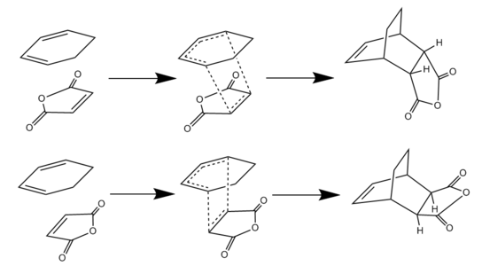 |
There have been many experimental examples [6] [7] that show the strongly favoured formation of the Endo product of the Diels Alder reaction under kinetic conditons. The reason for this is likely to be as a result of orbital interactions between the π system of the C=O groups on the maleic anhydride and the C=C π system on the cyclohexadiene. To investigate this 'Endo Rule' the transition structures and reaction pathways were investigated for both the endo and exo reaction (shown in diagram above). The method chosen consisted of modeling the desired endo and exo products in GaussView, optimising these structures to the ground state and then diliberately distorting this to a structure close to the TS. The transition structures were then calculated using the berny algorithm. All methods were carried out at the semi-empirical AM1 level of theory.
Locating the Transition Structure for the Formation of the Exo Product
The exo product was modeled and optimised at the semi-empirical AM1 level of theory. The results for this can be seen in the table below. The HOMO an LUMO of the molecule are also shown.
| Molecule | Structure | HOMO | LUMO | Calculation Summary | log. file | ||
|---|---|---|---|---|---|---|---|
| Exo Product |  |
 |
 |
log file |
In order to calculate the transition state structure, the optimised exo product structure was deliberately edited: both the C-C bonds connecting the starting molecules were deleted and the distance increased to approximately 2 Å. An optimisation to a transition structure using the Berny algorithm was then calculated. This proved successful in calculating a transition state structure, evidenced by the negative vibrational frequency mode at -812.20 cm-1 (indicative of a negative force constant and thus a maximum on the potential energy surface). The results and animations of the calculation can be seen below.
| Molecule | Structure | HOMO | LUMO | Calculation Summary | log. file | |||
|---|---|---|---|---|---|---|---|---|
| Exo TS |
|
 |
 |
 |
log file |
An intrinsic reaction coordinate calculation was carried out to verify the formation of the transition state. This can be seen below.
 |
 |
log file |
Locating the Transition Structure for the Formation of the Endo Product
In a similar fashion to the exo TS optimisation above, the endo TS was calculated first by optimising the endo-product structure. Secondly, this was deliberately distorted to allow a TS optimisation. The optimisation of ground state of the endo product can be seen below, along with the HOMO and LUMO.
| Molecule | Structure | HOMO | LUMO | Calculation Summary | log. file | ||
|---|---|---|---|---|---|---|---|
| Endo Product |  |
 |
 |
log file |
As in the case of the exo TS state, the bonds between the cyclohexene ring and the maleic anhydride were deleted and separation increased to approximately 2 Å. An optimisation to a TS was then carried out, again using the Berny algorithm. This proved successful in forming the TS structure, again evidenced by the negative vibrational frequency found at -806.06 cm-1.
| Molecule | Structure | HOMO | LUMO | Calculation Summary | log. file | |||
|---|---|---|---|---|---|---|---|---|
| Endo TS |
|
 |
 |
 |
log file |
Additionally, an intrinsic reaction coordinate calculation was carried out to verify the formation of the transition state. This can be seen below.
 |
 |
log file |
Comparison of Endo and Exo TS Structures and Energies
The optimised structures for the endo and exo transition states were compared in the table below. For the sake of clarity, only bond lengths and separations deemed of interest were included, however the original log files can be found in the tables above for completeness.
| Structure | Bond | Length/Å | Labeled Structure |
|---|---|---|---|
| Exo | C8-C10 | 1.41013 |  |
| C8-C6 | 2.17024 | ||
| C10-C12 | 2.17056 | ||
| C14-C3 | 2.94522 | ||
| C17-C2 | 2.94536 | ||
| H9-H22 | 2.89656 | ||
| H11-H23 | 2.89686 | ||
| H15-C3 | 2.41656 | ||
| H19-C2 | 2.41630 | ||
| Endo | C8-C12 | 2.16248 |  |
| C8-C6 | 1.40841 | ||
| C10-C6 | 2.16241 | ||
| C20-C3 | 2.89210 | ||
| C22-C3 | 2.89189 | ||
| H7-H16 | 2.23296 | ||
| H9-H19 | 2.23232 | ||
| H23-C2 | 3.08245 | ||
| H21-C3 | 3.08283 |
It can be seen that there are various similarities and differences between the two transition state stuctures. For example both the bond-breaking/making C-C separations were found to be very similar - 2.16 Å for endo and 2.17 Å for exo - though slightly short in the endo case. As expected, the main geometric differences can be found with the sp3-hybridised CH2 groups in the cylohexadiene ring. In the exo TS structure the H's nearest the maleic anhydride are 2.42 Å from the C of the C=O bond compared with 3.08 Å in the endo TS structure. This implies a greater steric hindrance between the -(C=O)-O-(C=O)-and the -CH2-CH2- in the exo product compared with the endo TS. Other relevant separations/bond lengths can also be seen in the table above.
The table below displays the electronic energies and thermochemical properties outputted from the optimisation reactions of the starting materials, TS structures and products. The results show that, using this level of theory, the endo and exo products have very similar electronic energies, however the endo product was found to be surprisingly lower in energy, indicating it to be the thermodynamic product. This contradicts most theory which predicts the exo to be thermodynamically stable [6].
(This is true for the general case, but in actuality the endo dominates for this particular reaction. Tam10 (talk) 15:47, 11 December 2015 (UTC))
| Semi-Empirical AM1 | |||
|---|---|---|---|
| Electronic energy | Sum of electronic and zero-point energies | Sum of electronic and thermal energies | |
| at 0 K | at 298.15 K | ||
| Cyclohexa-1,3-diene | 0.027711 | 0.152502 | 0.157726 |
| Maleic Anhydride | -0.121824 | -0.063346 | -0.058192 |
| Endo TS | -0.051505 | 0.133493 | 0.143683 |
| Exo TS | -0.050420 | 0.134880 | 0.144881 |
| Endo Product | -0.160171 | 0.031469 | 0.040468 |
| Exo Product | -0.159909 | 0.031701 | 0.040679 |
From the energies above it is possible to calculate the activation energies of the exo and endo reaction pathways, seen in the table below. The units are expressed in kcal/mol (1 Hartree = 627.509 kcal/mol ). The activation energies at 0 K are calculated from by the difference in energy between the sum of the electronic and zero-point energies for the reagents and the transition state structures. At 298.15 K the same was done however using the sum of electronic and thermal energies. Additionally, it is also possible to calculate the reaction energies. This was achieved using the same method as just mentioned with the exception that the difference in energy between the sum of the electronic and zero-point energies for the reagents and the products were considered. Theses are all displayed in the table below.
| Activation Energy at 0 K / kcal/mol | Activation Energy at 298.15 K / kcal/mol | Reaction Energy at 0 K / kcal/mol | Reaction Energy at 298.15 K / kcal/mol | |
|---|---|---|---|---|
| Endo | 27.822 | 27.704 | -36.199 | -37.064 |
| Exo | 28.692 | 28.456 | -36.054 | -36.932 |
At both temperatures, it is clear to see that the endo reaction pathway has a significantly lower energy barrier compared with the exo pathway. Consequently, it can be seen that during a kinetically controlled Diels Alder reaction, the kinetic product is the the endo product (for these reagents). The reason for this is postulated to be due to secondary orbital overlap between the -(C=O)-O-(C=O)-and the -CH-CH- π systems. However, it can be seen that in the HOMO of the endo TS structure, the -CH-CH- π orbitals are out of phase with the -(C=O)-O-(C=O)- π orbitals. Additionally, there is a nodal region between them, thus resulting in an unfavourable interaction. Thus, based on the calculations carried out at the semi-empirical level of theory, the secondary orbital interaction is unlikely to cause the stabilising effect that had been hoped for. However it would be worth investigating this using a higher level of theory in an effort to produce more accurate MOs.
Conclusion
The first part of this computational study investigated the reaction paths through which the Cope Rearrangement of 1,5-hexadiene takes place. Both the chair and boat transition state structures were modelled at both the HF/3-21G and B3LYP/6-31G* levels of theory, both of which afforded suitable geometries. It was seen that the chair transition state structure provided the lowest energy pathway with the smallest activation energy at both 0 K and 298.15 K.
Secondly, the a prototypic Diels Alder reaction between ethene and 1,3-butadiene was investigated. Initially the reagents were optimised (all parts of this section were computed using the semi-empirical AM1 level of theory in an effort to reduce the expense of the calculations) followed by TS optimisations. It was established that the reaction proceeded as would be expected through frontier molecular orbital theory/using the Woodward-Hoffmann rules.
The Diels Alder reaction between maleic anhydride and cyclohexa-1,3-dien was also investigated to establish the effect of substituents and secondary orbital interactions. The TS optimisation found the endo transition state structure to provide the lower energy, kinetically available reaction pathway. However, under analysis of the molecular orbitals it can be seen that there is no evidence of a secondary orbital interaction which would cause this, rather it is potentially down to the steric penalty of the CH2 groups in the exo product. It would be worth investigating this reaction using a higher level of theory to more accurately develop the molecular orbitals of the transition state structures.
References
- ↑ Mod:Phys3
- ↑ 2.0 2.1 Woodward, R.B.; Hoffmann, R.; Stereochemistry of Electrocyclic Reactions, J. Am. Chem. Soc.,1965, 87 (2), 395-397 DOI: 10.1021/ja01080a054
- ↑ [1] David C. Sherrill, An Introduction to Hartree-Fock Molecular Orbital Theory, 2001
- ↑ 4.0 4.1 [2] D. Nasipuri, Stereochemistry of Organic Compounds: Principles and Applications, 1994
- ↑ [doi:10.1351/goldbook.H02734 IUPAC.] Compendium of Chemical Terminology, 2nd ed. (the "Gold Book"). Compiled by A. D. McNaught and A. Wilkinson. Blackwell Scientific Publications, Oxford (1997).
- ↑ 6.0 6.1 James H. Cooley, Richard V. Williams, endo- and exo-Stereochemistry in the Diels–Alder Reaction: Kinetic versus Thermodynamic Control, J. Chem. Edu. 1997, 74, 582
- ↑ Ana Arrieta and Fernando P. Cossı́o, Direct Evaluation of Secondary Orbital Interactions in the Diels Alder Reaction between Cyclopentadiene and Maleic Anhydride, J. Org. Chem. 2001, 66, 6178-6180