Rep:Mod:Afg216CMP

CMP Modelling Computational Laboratory

Introduction

In this experiment, the Monte Carlo algorithm and the Ising Model of ferromagnetic materials are used to investigate energies and magnetisations of a two-dimensional ferromagnetic lattice. The model is used to predict the heat capacity, $C$, and Curie temperature, $T_C$, of the system. The Ising Model treats a ferromagnetic material as a simple lattice of magnetic spins, $s_i$, which can be either up or down - $s_i=\pm 1$; the lattice energy derives simply from the interactions of directly neighbouring spins and the lattice is treated as periodic - it repeats identically in all dimensions. Here a lattice in two dimensions only is used for simplicity of computation.

The Monte Carlo algorithm (voted the Top Algorithm of the 20th Century ) is used to significantly reduce the computational requirements of the situation such that it becomes reasonable to carry on a desktop computer. It does this by restricting the model to take only spin configurations which have above a certain threshold probability of existence, defined by the Boltzmann distribution (which uses the temperature at which the simulation is being run).

The Ising Model allows for the prediction and observation of the phase change that occurs at the Curie temperature, when it is used in two or more dimensions. The Curie temperature marks the point at which the competing energetic and entropic attributes of the system balance - just above absolute zero a system of magnetic spins will be aligned with all spins parallel (all with the same value of either $s_i=1$ or $s_i=-1$) as that is the lowest possible energy configuration. Above the Curie temperature, the system has enough thermal energy to overcome this energetic barrier and reorganise to maximise the entropy andd gain the energetic benefits associated with high entropy.

A range of lattice sizes and temperatures are tested and the magnetisations and energies associated with each investigated. From these simulations, heat specific capacities were extracted using the energies' variances and by extension the Curie temperatures of the system were approximated. From these values the Curie temperature of a real ferromagnetic material can be estimated and is done so, by extrapolating to an infinitely large Ising Lattice, which is a reasonable approximation.

Introduction to the Ising model: Tasks 1, 2 and 3

Task 1: Show that the lowest possible energy for the Ising model is $$\begin{gathered} E \\ = \\ -DNJ \end{gathered}$$, where $D$ is the number of dimensions and $N$ is the total number of spins. What is the multiplicity of this state? Calculate its entropy.

The lowest energy configuration of the Ising model has all spins parallel (all $s_i$ and $s_j$ with value 1 or -1). When this is the case,

$$\begin{gathered} \sum _{j \\ \in \\ \mathrm{n}\mathrm{e}\mathrm{i}\mathrm{g}\mathrm{h}\mathrm{b}\mathrm{o}\mathrm{u}\mathrm{r}\mathrm{s}\left(i\right)}{s}_i{s}_j \end{gathered}$$

becomes equal to the number of neighbours of each spin unit, as $s_i{s}_j$ becomes 1. Each spin unit in a $D-$ dimensional lattice has $2D$ immediately adjacent neighbours and thus:

$$\begin{gathered} \sum _{j \\ \in \\ \mathrm{n}\mathrm{e}\mathrm{i}\mathrm{g}\mathrm{h}\mathrm{b}\mathrm{o}\mathrm{u}\mathrm{r}\mathrm{s}\left(i\right)}{s}_i{s}_j=2D \end{gathered}$$

It follows that as

$\sum _i^N=N$

then, as the total expression for the energy is:

$$\begin{gathered} E=-\frac{1}{2}J\sum _i^N\sum _{j \\ \in \\ \mathrm{n}\mathrm{e}\mathrm{i}\mathrm{g}\mathrm{h}\mathrm{b}\mathrm{o}\mathrm{u}\mathrm{r}\mathrm{s}\left(i\right)}{s}_i{s}_j \end{gathered}$$

the energy in this minimum energy configuration can be expressed as:

$E=-\frac{1}{2}J\times N\times 2D$

(where the half prevents double counting of interactions) and thus:

$E=-DNJ$

as required. The multiplicity of this system is defined as the number of different ways of arranging the unit spins. As the spins are indistinguishable and all spins in this particular case are equal (at either 1 or -1) there are only two ways of arranging the system (where all spins are parallel or antiparallel) and as such the multiplicity, $\mathrm{\Omega }$ , is equal to 2. The entropy, $S$, of the system is given by the formula

$S=k_B\ln \mathrm{\Omega }$

where $k_B=1.38064852\times 10^{-23}{m}^{2}kg{s}^{-2}{K}^{-1}$, Boltzmann's Constant.

So, the entropy of this system where $\mathrm{\Omega }=2$ is given by:

$S=k_B\ln 2$

Task 2: Imagine that the system is in the lowest energy configuration. To move to a different state, one of the spins must spontaneously change direction ("flip"). What is the change in energy if this happens ($$\begin{gathered} D=3, \\ N=1000 \end{gathered}$$)? How much entropy does the system gain by doing so?

The energy of the system is given by:

$$\begin{gathered} E=-\frac{1}{2}J\sum _i^N\sum _{j \\ \in \\ \mathrm{n}\mathrm{e}\mathrm{i}\mathrm{g}\mathrm{h}\mathrm{b}\mathrm{o}\mathrm{u}\mathrm{r}\mathrm{s}\left(i\right)}{s}_i{s}_j \end{gathered}$$

Thus the energy difference between a system with all spins at 1 or -1 and a system with all but one spin at 1 or -1 and the other of the opposite spin to the rest is given by:

$$\begin{gathered} \mathrm{\Delta }E=(-\frac{1}{2}J\sum _i^N\sum _{j \\ \in \\ \mathrm{n}\mathrm{e}\mathrm{i}\mathrm{g}\mathrm{h}\mathrm{b}\mathrm{o}\mathrm{u}\mathrm{r}\mathrm{s}\left(i\right)}{s}_i{s}_j)-(-\frac{1}{2}J\sum _i^N\sum _{j \\ \in \\ \mathrm{n}\mathrm{e}\mathrm{i}\mathrm{g}\mathrm{h}\mathrm{b}\mathrm{o}\mathrm{u}\mathrm{r}\mathrm{s}\left(i\right)}{s}_i{s}_j) \end{gathered}$$

$$\begin{gathered} \mathrm{\Delta }E=(-\frac{1}{2}JN\sum _{j \\ \in \\ \mathrm{n}\mathrm{e}\mathrm{i}\mathrm{g}\mathrm{h}\mathrm{b}\mathrm{o}\mathrm{u}\mathrm{r}\mathrm{s}\left(i\right)}{s}_i{s}_j)-(-\frac{1}{2}JN\sum _{j \\ \in \\ \mathrm{n}\mathrm{e}\mathrm{i}\mathrm{g}\mathrm{h}\mathrm{b}\mathrm{o}\mathrm{u}\mathrm{r}\mathrm{s}\left(i\right)}{s}_i{s}_j) \end{gathered}$$

and this difference in interaction is $12J$ as, in three dimensions, each spin has 6 immediately adjacent neighbours. When one spin is flipped, six favourable parallel interactions are replaced by six unfavourable antiparallel interactions - a net interaction energy change of $12J$. Therefore:

$\mathrm{\Delta }E=12J$

The entropy change is given by:

$\mathrm{\Delta }S=k_B\ln {\mathrm{\Omega }}_{final}-k_B\ln {\mathrm{\Omega }}_{initial}=k_B(\ln (2(\genfrac{}{}{0ex}{}{1000}{1}))-\ln 2)$

$\mathrm{\Delta }S=k_B\ln 1000$

Task 3: Calculate the magnetisation of the 1D and 2D lattices in figure 1. What magnetisation would you expect to observe for an Ising lattice with $$\begin{gathered} D=3, \\ N=1000 \end{gathered}$$ at absolute zero?

The magnetisation, $M$, of the system is given by:

$M=\sum _i{s}_i$

Figure 1: Illustration of an Ising lattice in one (N=5), two (N=5x5), and three (N=5x5x5) dimensions. Red cells indicate the "up" spin", and blue cells indicate the "down" spin.

The respective magnetisations of the $D=1$ and $D=2$ lattices shown in Figure 1 are consequently as follows:

$M_{D=1}=\sum _i{s}_i=(3)\times (1)+(2)\times (-1)=1$

$M_{D=2}=\sum _i{s}_i=(4+3+3+2+1)\times (1)+(1+2+2+3+4)\times (-1)=1$

At absolute zero, you would expect the Ising lattice with $$\begin{gathered} D=3, \\ N=1000 \end{gathered}$$ to have magnetisation:

$M=\pm 1000$

depending on the direction that all spins in the lattice take - they should all be parallel at absolute zero as they do not have the thermal energy available to them that is required to overcome the energetic barrier associated with flipping spins.

Calculating the energy and magnetisation: Tasks 4 and 5

Task 4: Complete the functions energy() and magnetisation(), which should return the energy of the lattice and the total magnetisation, respectively.

Note: as suggested in the laboratory script, $J=1.0$ is assumed from here onwards as reduced units (in which $J=k_B$) are used.

The python script used to define the Ising Lattice object used in the experiment along with the first functions used to find the energy and magnetisation of the lattice are shown below.

import numpy as np

class IsingLattice:

    E = 0.0
    E2 = 0.0
    M = 0.0
    M2 = 0.0

    n_cycles = 0

    def __init__(self, n_rows, n_cols):
        self.n_rows = n_rows
        self.n_cols = n_cols
        self.lattice = np.random.choice([-1,1], size=(n_rows, n_cols))

    def energy(self):
        "Return the total energy of the current lattice configuration."
        J=1.0
        enesum=0
        for i in range(0,self.n_rows):
            for j in range(0,len(self.lattice[i])):                                                   #Here two loops are used to loop across every spin element in both dimensions.
                enesum=enesum+(self.lattice[i,j]*(self.lattice[i,(j-1)]+self.lattice[(i-1),j]))       #Here a loop is used to sum the vertical and horizontal interactions calculated for each spin element, with '-1' used to account for the periodic nature of the lattice
        energy = -1*J*enesum                                                                          #The sum of interactions is converted to a real energy value - 0.5 is not needed as the interactions are not double counted to reduce computational demand.
        return energy

    def magnetisation(self):
        "Return the total magnetisation of the current lattice configuration."
        magnetisation=0
        for i in range(0,self.n_rows):
            for j in range(0,len(self.lattice[i])):                                                   #The values of all spin elements are simply summed by looping across the rows and columns.
                magnetisation=magnetisation+self.lattice[i,j]
        return magnetisation

Task 5: Run the ILcheck.py script from the IPython Qt console using the command

%run ILcheck.py

The displayed window has a series of control buttons in the bottom left, one of which will allow you to export the figure as a PNG image. Save an image of the ILcheck.py output, and include it in your report.

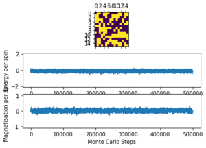
The results of the ILcheck.py script can be seen below in Figure 2. It shows that the energy and magnetisation functions shown above are functioning correctly by showing a maximum energy, minimum energy and random configuration of the lattice spins.

Figure 2: ILcheck.py results

Introduction to the Monte Carlo simulation: Tasks 6, 7 and 8

Task 6: How many configurations are available to a system with 100 spins? To evaluate these expressions, we have to calculate the energy and magnetisation for each of these configurations, then perform the sum. Let's be very, very, generous, and say that we can analyse $1\times 10^9$ configurations per second with our computer. How long will it take to evaluate a single value of ${⟨M⟩}_T$?

Each spin element can take two possible values ($s_i=\pm 1$) and thus the total number of spin configurations for a 10 by 10 element lattice is $2^{100}$ (as there are 100 spin elements). To calculate the expected or average magnetisation at a certain temperature, ${⟨M⟩}_T$, all of these configurations must be considered. Consequently, it would take:

$2^{100}$ configurations $÷1\times 10^9$ configurations per second $=1.27\times 10^{21}$seconds

to run through all configurations. This is obviously ludicrous given that the age of the universe is estimated to be $4.32\times 10^{17}$ seconds . This shows that the computational method must be improved - this is done by using the Monte Carlo algorithm, as discussed in the introduction.

Task 7: Implement a single cycle of the above algorithm in the montecarlocycle(T) function. This function should return the energy of your lattice and the magnetisation at the end of the cycle. You may assume that the energy returned by your energy() function is in units of $k_B$! Complete the statistics() function. This should return the following quantities whenever it is called: $<E>,<E^2>,<M>,<M^2>$, and the number of Monte Carlo steps that have elapsed.

Below the montecarlostep(T) and statistics() functions added to the IsingLattice object definition are shown. The algorithm functions by taking the starting spin configuration (defined by the __init__() function within the object), randomly flipping one spin and testing the configuration produced. The algorithm only accepts lattice configurations with energies lower than that which came before or with high enough probability of occurance when compared to the Boltzmann distribution - as the Boltzmann distribution is a function of temperature, which lattices would be accepted also depends on temperature. This generates a Boltzmann distributed set of lattice configurations from which the average energy and magnetisation can be calculated, and eliminates the need to consider every low probability configuration - which have negligible impact on the properties to be calculated - which in turn vastly reduces the computational demand of the experiment.

class IsingLattice:
.                                                                                     #The previous code within the IsingLattice object is as before.
.
.
    def montecarlostep(self, T):
        E0 = self.energy()
        random_i = np.random.choice(range(0, self.n_rows))
        random_j = np.random.choice(range(0, self.n_cols))
        self.lattice[random_i,random_j] = -1*self.lattice[random_i,random_j]          #This code chooses a random spin element in the lattice and flips its value.
        E1 = self.energy()
        random_number = np.random.random()
        dE = E1 - E0 
        if dE > 0: 
            if random_number > np.exp(-dE/T):                                         #This code chooses only high enough probability lattice configurations.
                self.lattice[random_i,random_j] = -1*self.lattice[random_i,random_j]  #This code restores the configuration if the new configuration was too unlikely. 
        self.n_cycles = self.n_cycles + 1
        self.E = self.E + self.energy()
        self.E2 = self.E2 + (self.energy())**2
        self.M = self.M + self.magnetisation()
        self.M2 = self.M2 + (self.magnetisation())**2                                 #This code updates the energy and magnetisation attributes of the lattice object after each step.
        return(self.energy(), self.magnetisation())
        
    def statistics(self):                                                             #This statistics() function calculates and returns the requested quantities at the end of each run.
        AvgE = self.E/self.n_cycles
        AvgE2 = self.E2/((self.n_cycles)**2)
        AvgM = self.M/self.n_cycles
        AvgM2 = self.M2/((self.n_cycles)**2)
        return (AvgE, AvgE2, AvgM, AvgM2, self.n_cycles)

Task 8: If $T<T_C$, do you expect a spontaneous magnetisation (i.e. do you expect $⟨M⟩\ne 0$)? When the state of the simulation appears to stop changing (when you have reached an equilibrium state), use the controls to export the output to PNG and attach this to your report. You should also include the output from your statistics() function.

Theoretically, spontaneous magnetisation is indeed expected below $T_C$ as the energetic cost of flipping the spins to maximise the system entropy is too great compared to the amount of thermal energy the system has - the system will align the spins and as such show a magnetisation, $⟨M⟩$, of greater or less than zero. Quantitatively, this can be explained using Helmholtz Free Energy, $A$, and the fact that the system always looks to minimise it. Helmholtz Free Energy is given by:

$A=U-TS$

and thus when $T$ is low, the entropy has a much lower impact on $A$ than $U$, the internal energy. This can be used to quantitatively find the tipping point $T_C$ above which the system adjusts to maximise entropy.

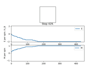
Below in Figures 3 and 4 the ILanim.py results are shown. Note - ILanim.py had to be run on a different computer due to technical difficulties, hence the lines within the code screenshot indicating that it has been run by someone else. It can be seen that a minimum energy has been reached at this temperature (which must be below $T_C$ as the system has reached equilibrium (all spins in the lattice have aligned and are parallel); a maximum magnetisation has also been reached for the same reason.

Figure 3: Screenshot of equilibrated 8x8 lattice at 1 K

Figure 4: Screenshot of statistics generated by ILanim.py

Accelerating the Code: Tasks 9, 10 and 11

Task 9: Use the script ILtimetrial.py to record how long your current version of IsingLattice.py takes to perform 2000 Monte Carlo steps. This will vary, depending on what else the computer happens to be doing, so perform repeats and report the error in your average!

10 Runs of the ILtimetrial.py script were carried out to account for fluctuations in performance due to differing background operations:

%run ILtimetrial
Took 6.491240794751832s

%run ILtimetrial
Took 6.198033647801431s

%run ILtimetrial
Took 6.39347229230993s

%run ILtimetrial
Took 6.2046913622484325s

%run ILtimetrial
Took 6.873771136789344s

%run ILtimetrial
Took 6.258122856385299s

%run ILtimetrial
Took 6.286337743869581s

%run ILtimetrial
Took 6.719355183591773s

%run ILtimetrial
Took 6.612273236569536s

%run ILtimetrial
Took 6.688410581865767s

Quantity	Value
Mean Time / s	6.47
Standard Deviation	0.229

This time trial data shows the inefficiencies present in that particular iteration of the IsingLattice object code; it is always desirable to run simulations as quickly as possible and improvements were then made.

Task 10: Look at the documentation for the NumPy sum function. You should be able to modify your magnetisation() function so that it uses this to evaluate M. The energy is a little trickier. Familiarise yourself with the NumPy roll and multiply functions, and use these to replace your energy double loop (you will need to call roll and multiply twice!).

The efficiency of the energy() and magnetisation() functions could be improved significantly; the resulting code is shown below.

class IsingLattice:
.
.
. 
    def energy(self):
        "Return the total energy of the current lattice configuration."
        J=1
        up = np.roll(self.lattice, 1, axis=0)
        side = np.roll(self.lattice, 1, axis=1)                               #This code duplicates the spin lattice and moves it up and right respectively.
        upE = np.multiply(up, self.lattice)
        sideE = np.multiply(side, self.lattice)                               #This code multiplies the original lattice with the 'up' and 'side' lattices respectively.
        totalE = -J*(upE + sideE)                                             #This code sums the interaction lattices and multiplies the summed lattice by J to give the real energy.
        return np.sum(totalE)

    def magnetisation(self):
        "Return the total magnetisation of the current lattice configuration."
        return np.sum(self.lattice)                                           #This code sums all elements in the lattice succintly to give the overall magnetisation.

Task 11: Use the script ILtimetrial.py to record how long your new version of IsingLattice.py takes to perform 2000 Monte Carlo steps. This will vary, depending on what else the computer happens to be doing, so perform repeats and report the error in your average!

10 further runs of the ILtimetrial.py script were carried out to account for fluctuations in performance due to differing background operations:

 %run ILtimetrial.py
Took 0.36230830418159893s

%run ILtimetrial.py
Took 0.3577631995347126s

%run ILtimetrial.py
Took 0.3494842495103363s

%run ILtimetrial.py
Took 0.3503130425857659s

%run ILtimetrial.py
Took 0.35432486293695487s

%run ILtimetrial.py
Took 0.3491284415440008s

%run ILtimetrial.py
Took 0.3588639804305611s

%run ILtimetrial.py
Took 0.3561783145308208s

%run ILtimetrial.py
Took 0.36012299323451735s

%run ILtimetrial.py
Took 0.35134796479554s

Quantity	Value
Mean Time / s	0.355
Standard Deviation	0.00452

The obvious significant reduction in average processing time (by 18.2 times) shows the dramatic increase in computational efficiency facilitated by the code change above.

The Effect of Temperature: Tasks 12 and 13

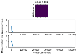
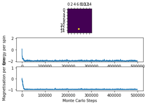
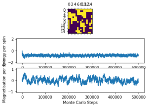
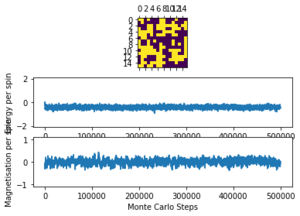
Task 12: The script ILfinalframe.py runs for a given number of cycles at a given temperature, then plots a depiction of the final lattice state as well as graphs of the energy and magnetisation as a function of cycle number. This is much quicker than animating every frame! Experiment with different temperature and lattice sizes. How many cycles are typically needed for the system to go from its random starting position to the equilibrium state? Modify your statistics() and montecarlostep() functions so that the first N cycles of the simulation are ignored when calculating the averages. You should state in your report what period you chose to ignore, and include graphs from ILfinalframe.py to illustrate your motivation in choosing this figure.

The simulations run to investigate the variation of equilibration time with lattice size can be seen below.

Temperature / K	Lattice Size	Approximate no. Cycles to Equilibration	.png Graphic
1.0	2x2	100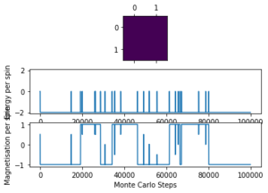
1.0	4x4	200
1.0	8x8	1000
1.0	16x16	8000
1.0	32x32	80000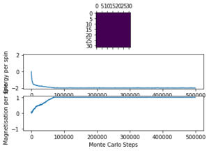

The simulations run to investigate the variation in equilibration time with temperature can be seen below.

Temperature / K	Lattice Size	Approximate no. Cycles to Equilibration	.png Graphic
0.5	16x16	10000
1.0	16x16	8000
1.5	16x16	10000
2.0	16x16	20000
3.0	16x16	20000
4.0	16x16	5000
5.0	16x16	0
10.0	16x16	0
15.0	16x16	0
20.0	16x16	0

From this data it is easier to observe that at some point between 2 K and 3 K the Curie temperature is surpassed - at 3 K the system is high in entropy and lower in internal energy but at 2 K the entropy is minimised and the internal energy is maximised by aligning spins. At 3 K and above the magnetisation fluctuates around an equilibrium value of 0 but below it fluctuates around equilibrium non-zero values. It can also be seen that at higher temperatures more 'noise' due to thermal fluctuations is seen and that larger lattices appear to take longer to equilibrate in general (as the flipping of one spin has less of an impact on the whole systems when there are more spin elements in the system), although at higher temperatures this effect is reduced as the lattices begin approximately in equilibrium (as the random starting configuration is more likely to be around equilibrium at higher temperatures).

The modified code which accounts for the delay in equilibration is shown below.

    def montecarlostep(self, T):
        "Performs 1 Monte Carlo step on the given lattice and updates the attributes of the lattice accordingly."
        E0 = self.energy()
        random_i = np.random.choice(range(0, self.n_rows))
        random_j = np.random.choice(range(0, self.n_cols))
        self.lattice[random_i,random_j] = -1*self.lattice[random_i,random_j]
        E1 = self.energy()
        random_number = np.random.random()
        dE = E1 - E0 
        if dE > 0: 
            if random_number > np.exp(-dE/T):
                self.lattice[random_i,random_j] = -1*self.lattice[random_i,random_j]
        self.n_cycles = self.n_cycles + 1                                               #Up to here, the code is the same as before.
        equilibrationdelay = N                                                          #The equilibration delay cycle number is defined here.
        if self.n_cycles > equilibrationdelay:                                          #The code from here stops the statistics being recorded until the equilibration delay is passed.
            self.E = self.E + self.energy()
            self.E2 = self.E2 + (self.energy())**2
            self.M = self.M + self.magnetisation()
            self.M2 = self.M2 + (self.magnetisation())**2
        return(self.energy(), self.magnetisation())
        
    def statistics(self):
        "Returns the statistics associated with the Monte Carlo steps performed."
        equilibrationdelay = N                                                          #The equilibration delay is also defined here.
        AvgE = self.E/(self.n_cycles-equilibrationdelay)                                #The adjustment for the delay in the statistics is here.
        AvgE2 = self.E2/((self.n_cycles-equilibrationdelay)**2)
        AvgM = self.M/(self.n_cycles-equilibrationdelay)
        AvgM2 = self.M2/((self.n_cycles-equilibrationdelay)**2)
        return (AvgE, AvgE2, AvgM, AvgM2, self.n_cycles)

From here on an equilibration delay is taken to be 10,000, as for the relevant lattice sizes and temperatures investigated this accounts for equilibration. The downsides to this assumption are discussed later.

Task 13: Use ILtemperaturerange.py to plot the average energy and magnetisation for each temperature, with error bars, for an $8\times 8$ lattice. Use your intuition and results from the script ILfinalframe.py to estimate how many cycles each simulation should be. The temperature range 0.25 to 5.0 is sufficient. Use as many temperature points as you feel necessary to illustrate the trend, but do not use a temperature spacing larger than 0.5. The NumPy function savetxt() stores your array of output data on disk — you will need it later. Save the file as 8x8.dat so that you know which lattice size it came from.

The code used to plot the required graph (of energy per spin against temperature for an 8x8 Ising Lattice) is shown below.

eight1 = loadtxt("8x8_temprange_0.2to5_0.1int_100000steps_delay10000.dat")          #Loading the relevant simulation files
eight2 = loadtxt("8x8_temprange_0.2to5_0.1int_100000steps_delay10000_2.dat")
eight3 = loadtxt("8x8_temprange_0.2to5_0.1int_100000steps_delay10000_3.dat")
eight4 = loadtxt("8x8_temprange_0.2to5_0.1int_100000steps_delay10000_4.dat")
eight5 = loadtxt("8x8_temprange_0.2to5_0.1int_100000steps_delay10000_5.dat")

def temprange(file):                                                                #Defining functions to extract the required data from the files.
    'Retrieves temperature range from given file.'
    temps = file[:,0]
    return temps

def avgEs(file):
    'Returns average energies at each temp from given file.'
    avges = file[:,1]
    return avges

def avgE2s(file):
    'Returns average energies squared at each temp from given file.'
    avge2s = file[:,2]
    return avge2s

def avgMs(file):
    'Returns average magnetisations at each temp from given file.'
    avgMs = file[:,3]
    return avgMs

def avgM2s(file):
    'Returns average magnetisations squared at each temp from given file.'
    avgM2s = file[:,4]
    return avgM2s

stdvals = []                                                                          #Generating a list of standard deviation values.
for i in range(0,len(avgEs(eight1))):
    val0=[avgEs(eight1)[i],avgEs(eight2)[i],avgEs(eight3)[i],avgEs(eight4)[i],avgEs(eight5)[i]]
    stddevval=[np.std(val0)]
    stdvals=stdvals+stddevval

AverageEnergies = (avgEs(eight1)+avgEs(eight2)+avgEs(eight3)+avgEs(eight4)+avgEs(eight5))/5
temps = temprange(eight1)                                                             #Creating a list of average energies from the repeats run.

xlabel('Temperature / K')
ylabel('Average Energy per Spin / J kB')
title('The Relationship Between Temperature and Energy per Spin of an 8x8 Lattice with Error Bars')
errorbar(temps,AverageEnergies,stdvals,None,linestyle='none',marker='.')              #Plotting the required graph with error bars generated from the repeat runs.
show()

stdvals = []
for i in range(0,len(avgMs(eight1))):
    val0=[avgMs(eight1)[i],avgMs(eight2)[i],avgMs(eight3)[i],avgMs(eight4)[i],avgMs(eight5)[i]]
    stddevval=[np.std(val0)]
    stdvals=stdvals+stddevval                                                         #Generating the equivalent standard deviation list but for magnetisation.
    
AverageMagnetisations = (avgMs(eight1)+avgMs(eight2)+avgMs(eight3)+avgMs(eight4)+avgMs(eight5))/5
                                                                                      #Creating an equivalent average value list for magnetisation.
xlabel('Temperature / K')
ylabel('Average Magnetisation per Spin')
title('The Relationship Between Magnetisation and Energy per Spin of an 8x8 Lattice with Error Bars')
errorbar(temps,AverageMagnetisations,stdvals,None,linestyle='none',marker='.')        #Plotting the equivalent graph for magnetisation.
show()

The generated graphs are shown below in Figures 5 and 6. They were generated by performing 100,000 Monte Carlo cycles on an 8x8 Ising Lattice at temperature intervals of 0.1 K from 0.2 K to 5 K.

Figure 5: Energy per Spin against Temperature with Error Bars.

Figure 6: Magnetisation per Spin against Temperature with Error Bars.

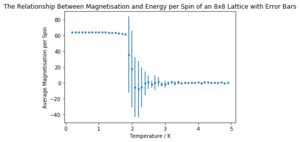
It can be easily seen that the energy per spin in the system increases with temperature. The standard deviation is much higher in the transition region (between entropic and energetically controlled equilibria) anchored around the Curie temperature. The magnetisation per spin is near 1 at low temperatures (below the Curie temperature) but decreases dramatically above $T_C$ to settle around zero as the system is no longer spontaneously magnetised, as discussed earlier. Note that the graphs have not been normalised to lattice size due to an error in the code - the 8x8 lattice graph here shows values 64 times larger than they should be.

The Effect of System Size: Task 14

Task 14: Repeat the final task of the previous section for the following lattice sizes: 2x2, 4x4, 8x8, 16x16, 32x32. Make sure that you name each datafile that your produce after the corresponding lattice size! Write a Python script to make a plot showing the energy per spin versus temperature for each of your lattice sizes. Hint: the NumPy loadtxt function is the reverse of the savetxt function, and can be used to read your previously saved files into the script. Repeat this for the magnetisation. As before, use the plot controls to save your a PNG image of your plot and attach this to the report. How big a lattice do you think is big enough to capture the long range fluctuations?

The same simulation as before (0.2 to 5 K in steps of 0.1, 10000 equilibration delay and 100000 total cycles) was carried out for 2x2, 4x4, 16x16 and 32x32 element lattices. Only three repeats of each lattice size were carried out due to time constraints.

It can be seen that the long range fluctuations become less significant as the lattice size increases. It appears that the 16x16 lattice is the smallest lattice in which the long range fluctuations can be obviously observed.

A sample of the code used to plot the required graphs is shown below. As before, there is a normalisation factor missing in the code and as such the values should be divided by their number of elements (i.e. 2x2 by 4, 4x4 by 16 etc.).

four1 = loadtxt("4x4_temprange_0.2to5_0.1int_100000steps_delay10000.dat")
four2 = loadtxt("4x4_temprange_0.2to5_0.1int_100000steps_delay10000_2.dat")
four3 = loadtxt("4x4_temprange_0.2to5_0.1int_100000steps_delay10000_3.dat")

stdvals = []
for i in range(0,len(avgEs(four1))):
    val0=[avgEs(four1)[i],avgEs(four2)[i],avgEs(four3)[i]]
    stddevval=[np.std(val0)]
    stdvals=stdvals+stddevval

AverageEnergies = (avgEs(four1)+avgEs(four2)+avgEs(four3))/3
temps = temprange(four1)

xlabel('Temperature / K')
ylabel('Average Energy per Spin / J kB')
title('The Relationship Between Temperature and Energy per Spin of a 4x4 Lattice with Error Bars')
errorbar(temps,AverageEnergies,stdvals,None,linestyle='none',marker='.')
show()

stdvals = []
for i in range(0,len(avgMs(four1))):
    val0=[avgMs(four1)[i],avgMs(four2)[i],avgMs(four3)[i]]
    stddevval=[np.std(val0)]
    stdvals=stdvals+stddevval

AverageMagnetisations = (avgMs(four1)+avgMs(four2)+avgMs(four3))/3

xlabel('Temperature / K')
ylabel('Average Magnetisation per Spin')
title('The Relationship Between Temperature and Magnetisation per Spin of a 4x4 Lattice with Error Bars')
errorbar(temps,AverageMagnetisations,stdvals,None,linestyle='none',marker='.')
show()

The graphs reflecting the effect of lattice size are shown below.

Lattice Size	Energy per Spin Graph	Magnetisation per Spin Graph
2x2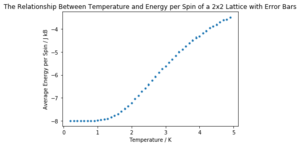
4x4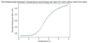
8x8
16x16
32x32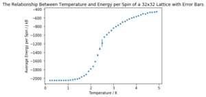

Determining the Heat Capacity: Tasks 15 and 16

Task 15: By definition,

$C=\frac{\partial ⟨E⟩}{\partial T}$

From this, show that

$C=\frac{\mathrm{V}\mathrm{a}\mathrm{r}[E]}{k_B{T}^2}$

(Where $\mathrm{V}\mathrm{a}\mathrm{r}[E]$ is the variance in $E$.)

To begin:

$U=⟨E⟩$

The variance in $U$ can be defined as the rate of change of $U$ undergoing thermal fluctuations. Thus:

$\mathrm{V}\mathrm{a}\mathrm{r}[U]=-\frac{\partial U}{\partial \beta }$

where $\beta =\frac{1}{k_{B}T}$. The heat capacity, $C$, of the system is defined as:

$C=\frac{\partial U}{\partial T}$

So, by extension (and the product rule):

$C=\frac{\partial U}{\partial T}=\frac{\partial U}{\partial \beta }\frac{\partial \beta }{\partial T}$

and since we have:

$\frac{\partial U}{\partial \beta }=-\mathrm{V}\mathrm{a}\mathrm{r}[U];\frac{\partial \beta }{\partial T}=-\frac{1}{k_B{T}^2}$

we can conclude that:

$C=\frac{\mathrm{V}\mathrm{a}\mathrm{r}[E]}{k_B{T}^2}$

as required.

Task 16: Write a Python script to make a plot showing the heat capacity versus temperature for each of your lattice sizes from the previous section. You may need to do some research to recall the connection between the variance of a variable, $\mathrm{V}\mathrm{a}\mathrm{r}[X]$, the mean of its square $⟨X^2⟩$, and its squared mean ${⟨X⟩}^2$. You may find that the data around the peak is very noisy — this is normal, and is a result of being in the critical region. As before, use the plot controls to save your a PNG image of your plot and attach this to the report.

Lattice Size	Heat Capacity Graph
2x2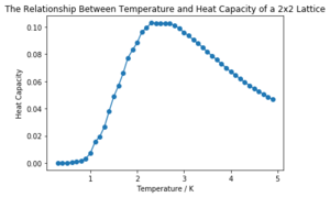
4x4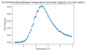
8x8
16x16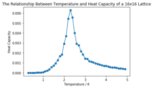
32x32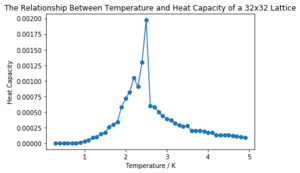

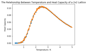
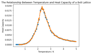
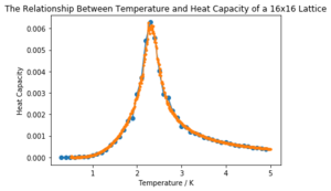
It can be seen that the larger the lattice size, the sharper the heat capacity peak (which occurs at the Curie temperature) and the greater the error around the peak. Ideally more temperature values within the range would have been used to smooth the peaks somewhat, but time was restricted.

The script used to calculate and plot heat capacity against temperature for the different lattice sizes is shown below. The factors used to convert the heat capacities form heat capacity per spin to heat capacity of the whole lattice are added into the code (and are simply the number of spins in the lattice, i.e. 2x2 has a factor of 4). The data used is averaged across three simulation runs of each size. Note that errors in the calculation of the squared energy and magnetisation (time restricted the amendment of the IsingLattice.py file and rerunning of the simulations) values when running the simulations are accounted for by the 90,000 (the number of cycles across which the average was taken) multiplication.

def heatcapacity(file,latticedimension):
    'Plots a graph of heat capacity against temperature from a given file.'
    Temps=temprange(file)
    E=avgEs(file)/(latticedimension**2)
    E2=(avgE2s(file)*90000)/(latticedimension**2 * latticedimension**2)
    VarE = E2 - (E**2)
    HeatCapacities = VarE / Temps**2
    return HeatCapacities

twoav=(two1+two2+two3)/3
fourav=(four1+four2+four3)/3
eightav=(eight1+eight2+eight3)/3
sixtav=(sixt1+sixt2+sixt3)/3
thirav=(thir1+thir2+thir3)/3

xlabel('Temperature / K')
ylabel('Heat Capacity')
title('The Relationship Between Temperature and Heat Capacity of a 2x2 Lattice')
plot(temprange(two1)[1:], heatcapacity(twoav, 2)[1:]*(2*2), marker="o")
show()
.
.
.
xlabel('Temperature / K')
ylabel('Heat Capacity')
title('The Relationship Between Temperature and Heat Capacity of a 32x32 Lattice')
plot(temprange(thir1)[1:], heatcapacity(thirav, 32)[1:]*(32*32), marker="o")
show()

Locating the Curie Temperature: Tasks 17, 18, 19 and 20

Task 17: A C++ program has been used to run some much longer simulations than would be possible on the college computers in Python. You can view its source code here if you are interested. Each file contains six columns: $T,E,E^2,M,M^2,C$ (the final five quantities are per spin), and you can read them with the NumPy loadtxt function as before. For each lattice size, plot the C++ data against your data. For one lattice size, save a PNG of this comparison and add it to your report — add a legend to the graph to label which is which. To do this, you will need to pass the label="..." keyword to the plot function, then call the legend() function of the axis object (documentation here).

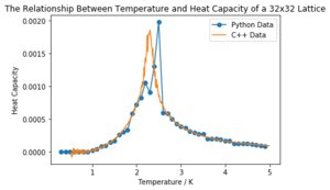
The heat capacity calculated above in python of a 4x4 lattice is plotted against that given, calculated in C++, below in Figure 7. Note that the heat capacities were originally calculated per spin, but, as above, here they represent those of the full lattices and the respective factors can be seen again in the code. All of the lattice sizes matched the C++ data fairly well (and can be seen in the 'CMP Modelling.ipynb' notebook attached). The 32x32 lattice size matched the least well, likely due to the larger uncertainty associated with the region around the peak; it fit better with the averaged data rather than with any individual run, proving the usefulness of repeats.

Figure 7: Heat capacity of a 2x2 lattice as calculated in Python and in the given C++ data

Figure 8: Heat capacity of a 4x4 lattice as calculated in Python and in the given C++ data

Figure 9: Heat capacity of a 8x8 lattice as calculated in Python and in the given C++ data

Figure 10: Heat capacity of a 16x16 lattice as calculated in Python and in the given C++ data

Figure 11: Heat capacity of a 32x32 lattice as calculated in Python and in the given C++ data

The plot code is shown here with the 4x4 size used as an example.

FourCpl = loadtxt("Cpl4x4.dat")                                                                  #Loading the C++ data.

xlabel('Temperature / K')
ylabel('Lattice Heat Capacity')
title('The Relationship Between Temperature and Heat Capacity of a 4x4 Lattice')
plot(temprange(four1)[1:], heatcapacity(four1, 4)[1:]*(4*4), marker="o", label="Python Data")    #Plotting the python data.
plot(temprange(FourCpl)[1:], FourCpl[1:, 5], marker=".", label='C++ Data')                       #Plotting the C++ data.
legend(loc="upper right")                                                                        #Adding a legend.
show()

Task 18: Write a script to read the data from a particular file, and plot C vs T, as well as a fitted polynomial. Try changing the degree of the polynomial to improve the fit — in general, it might be difficult to get a good fit! Attach a PNG of an example fit to your report.

The code used to plot the C vs T points and a polynomial fit to the points for the 4x4 lattice is shown below.

T = fourav[:,0]                                                                 #Generating the temperature range from the averaged data 'fourav'.
C = heatcapacity(fourav, 4)                                                     #Generating the heat capacity data from 'fourav'.
fit = np.polyfit(T, C*(4*4), 15)                                                #Fitting with a 15 order polynomial.
T_min = np.min(T)                                                               #Setting the range of the fit points as the full range of the data.
T_max = np.max(T)
T_range = np.linspace(T_min, T_max, 1000)
fitted_C_values = np.polyval(fit, T_range)
xlabel('Temperature / K')
ylabel('Heat Capacity')
title('Heat Capacity Against Temperature and Polynomial Fit for a 4x4 Lattice')
plot(T,C*(4*4), marker='.', linestyle='None')                                   #Plotting the python data.
plot(T_range, fitted_C_values, marker='', linestyle='-')                        #Plotting the polynomial fit.
show()

The requisite graph for the 4x4 lattice is shown below in Figure 12.

Figure 12: Heat capacity of a 4x4 lattice as calculated in Python and a polynomial fit of the points of order 15.

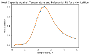
The rest of the fits are shown in the notebook 'CMP Modelling.ipynb' attached. In general, higher order polynomials garnered a better fit for all lattice sizes. The fits for the 32x32 lattice and 16x16 lattice are much worse, even at higher orders, but they were improved in the next task.

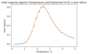
Task 19: Modify your script from the previous section. You should still plot the whole temperature range, but fit the polynomial only to the peak of the heat capacity! You should find it easier to get a good fit when restricted to this region.

The modified code is shown below with the 4x4 used as an example.

T = fourav[:,0]
C = heatcapacity(fourav, 4)
fit = np.polyfit(T, C*(4*4), 15)
T_min = 1                                           #These set the minimum and maximum values of the range for the fit.
T_max = 4
T_range = np.linspace(T_min, T_max, 1000)
fitted_C_values = np.polyval(fit, T_range)
C4max = np.max(fitted_C_values)
T4max = T_range[fitted_C_values == C4max]           #This code retrieves the maximum value of C and the corresponding value of T.
xlabel('Temperature / K')
ylabel('Heat Capacity')
title('Heat Capacity Against Temperature and Polynomial Fit for a 4x4 Lattice')
plot(T,C*(4*4), marker='.', linestyle='None')
plot(T_range, fitted_C_values, marker='', linestyle='-')
show()

The fit within the restricted range is shown below in Figure 13. Note that due to high uncertainty in the critical region around the Curie temperature we cannot have great confidence in the fits. Particularly for smaller lattice sizes the fits do seem overtly adequate, but the larger lattices (namely 16x16 and 32x32) still do not fit very well with the simulation data.

Figure 13: Heat capacity of a 4x4 lattice as calculated in Python and a restricted range polynomial fit to the points of order 15.

Task 20: Find the temperature at which the maximum in C occurs for each datafile that you were given. Make a text file containing two columns: the lattice side length (2,4,8, etc.), and the temperature at which C is a maximum. This is your estimate of $T_C$ for that side length. Make a plot that uses the scaling relation given above to determine $T_{C,\mathrm{\infty }}$. By doing a little research online, you should be able to find the theoretical exact Curie temperature for the infinite 2D Ising lattice. How does your value compare to this? Are you surprised by how good/bad the agreement is? Attach a PNG of this final graph to your report, and discuss briefly what you think the major sources of error are in your estimate.

Lattice Size	CMax	TC
2x2	0.4151056	2.4958959
4x4	0.8083970	2.4654655
8x8	1.1525856	2.3687688
16x16	1.3887500	2.3073073
32x32	1.2552730	2.3663664

The code used to plot the graph from which the Curie temperature of a theoretical infinite lattice could be extrapolated is shown below. In fitting, the first and last points (from the 2x2 and 32x32 lattices) were left out as both seemed anomalous.

Tfit = np.polyfit(invCTlatticevals[1:4], invCTtempvals[1:4], 1)
Lrange = np.linspace(0, 0.5, 1000)

fitted_T_values = np.polyval(fit, T_range)
xlabel('1 / Lattice Dimension')
ylabel('Curie Temperature Estimate / K')
title('Curie Temperature Vs. the Reciprocal of Lattice Size with a Linear Fit')
plot((invCTlatticevals), invCTtempvals, marker='.', linestyle='None')
plot(Lrange, (Tfit[0]*Lrange + Tfit[1]), marker='', linestyle='-')
show()
print(Tfit[1])

The y intercept on the graph corresponds to the value of the Curie temperature of an infinitely large lattice, as demonstrated by the scaling relation:

$T_{C,L}=\frac{A}{L}+T_{C,\mathrm{\infty }}$

The y intercept, $T_{C,\mathrm{\infty }}$, is given by the print command at the end of the above code. The extrapolated value was 2.259. The graph is shown below in Figure 14.

Figure 14: Curie temperature against reciprocal of lattice size with a linear fit.

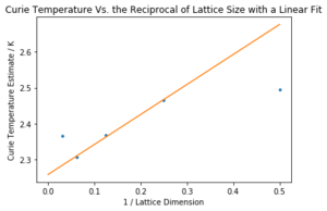
This compares favourably with the literature value of 2.269). The relative error is only 0.441 %. Given the many sources of error (including the error in polynomial fits and the high errors in the critical regions of the measurements) this seems a very reasonable result. The experiment would have been improved by taking more temperature points in the original runs to improve resolution, by taking measurements from more lattice sizes (as a fit of only three points is never ideal), by taking more repeats to lessen the impact of the error in the critical region (which was unfortunately not possible here due to time restraints), by improving the equilibration delay code (which was done visually with no real quantitative justification) or by using a more efficient processing language than python - the C++ data was much more extensive and proved the usefulness in using another language, particularly in the reduuction of run time, allowing for more repeats and smoother data to be acquired. In order to improve the equilibration delay code, there might have been a way to automate the delay to remove some of the qualitative error in looking for the point of equilibration. That also would have allowed for different delays to be used for the different lattice sizes which would again have improved the experiment. This might have been done by assessing the standard deviation of points within a range, and only taking the statistics data once it had fallen below a set value, representing the extent of fluctuations at equilibrium.

Conclusion

The simulations successfully yielded results comparable to those in the literature; the experiment was very successful bearing in mind the scope for error involved and the lack of repitition within it. The results were found quickly and with relative ease and as such reflected the useful (and transferable) nature of the python programming language within scientific computation. In practice, a much broader range of values and a much greater number of runs should be carried out to improve the experiment such that it can be treated as reliable.

References

- ↑ F. Bresme, O. Robotham, "Third Year CMP Compulsory Experiment Lab Script", https://wiki.ch.ic.ac.uk/wiki/index.php?title=Third_year_CMP_compulsory_experiment, accessed 20/11/2018
- ↑ J. Dongarra , F. Sullivan, "Guest Editors Introduction to the Top 10 Algorithms", Computing in Sci. and Eng., 2000, 2, 22-23.DOI:10.1109/MCISE.2000.814652
- ↑ P. Atkins, J. de Paula, "Atkins' Physical Chemistry", ISBN : 978-0-19-969740-3
- ↑ Physicsoftheuniverse.com, "The Universe by Numbers", https://www.physicsoftheuniverse.com/numbers.html, accessed 15/11/2018
- ↑ J. Kotze, "An Introduction to Monte Carlo Methods for an Ising Model of a Ferromagnet", 2008, 22, https://arxiv.org/pdf/0803.0217.pdf