Rep:Mod:AM6013
Introduction to molecular dynamics simulation
TASK: Open the file HO.xls. In it, the velocity-Verlet algorithm is used to model the behaviour of a classical harmonic oscillator. Complete the three columns "ANALYTICAL", "ERROR", and "ENERGY": "ANALYTICAL" should contain the value of the classical solution for the position at time , "ERROR" should contain the absolute difference between "ANALYTICAL" and the velocity-Verlet solution (i.e. ERROR should always be positive -- make sure you leave the half step rows blank!), and "ENERGY" should contain the total energy of the oscillator for the velocity-Verlet solution. Remember that the position of a classical harmonic oscillator is given by (the values of , , and are worked out for you in the sheet).
To calculate the classical solution of the position, the corresponding values of t were substituted in the given equation. The values for , , and were all equal to 1, except for , which was equal to 0. So, for example, at time 1.00:
To calculate the error, the absolute value of the difference between 'ANALYTICAL' and the velocity-Verlet Alogarithm was taken. The error was found to be small, of the order of 10E-03, meaning that the classical harmonic osciallator is a good approximation of the velocity-Verlet approximation. As can be seen in Figure 1, the values for both solutions fall almost perfectly on top of each other, confirming that the classical harmonic oscillator is a really good approximation. Figure 2 shows how the error increases with time.


For the energy calculation (i.e. sum of kinetic and potential energy), the following formula was used , where both and were the results from the velocity-Verlet approximation. The firs term corresponds to the kinetic energy and the second term to the potential energy. It was found that the energy stayed relatively constant throughout the whole simulation.
TASK: For the default timestep value, 0.1, estimate the positions of the maxima in the ERROR column as a function of time. Make a plot showing these values as a function of time, and fit an appropriate function to the data.
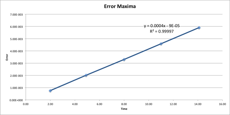
When plotting the maxima in the error as a function of time, the following graph is obtained. It can be clearly seen that the error gets bigger with time in a linear way.
TASK: Experiment with different values of the timestep. What sort of a timestep do you need to use to ensure that the total energy does not change by more than 1% over the course of your "simulation"? Why do you think it is important to monitor the total energy of a physical system when modelling its behaviour numerically?
One of the constraints in the simulation is that the total energy of the system has to remain constant, therefore it is important to monitor the energy to make sure this constraint is meet for the simulation to give valid results. If the system is not in equilibrium the results we would get wouldn't be useful and running the simulation would be pointless. We want the system to be in equilibrium because that's what real systems tend to be at. For the total energy not to change be more than 1% over the course of the simulation, the timestep has to be set to 2.00.
TASK: For a single Lennard-Jones interaction, , find the separation, , at which the potential energy is zero. What is the force at this separation? Find the equilibrium separation, , and work out the well depth (). Evaluate the integrals , , and when .
For the potential to be zero, since is contant, the term has to be zero. Therefore,
→
These two terms will be equal when , and so at this distance the potential energy will be zero.
To find out the force at this separation, we know that so by derivating the potential energy with respect to distance we get :
and because it's been established that, we can modify the expression to get
→→
To work out the equilibrium separation (i.e.when F=0), we know the term has to be zero so,
→→
To find the well depth when r is equal to the equilibrium distance we substitute all the 'r's for the value of the distance when F=0,
Therefore when the two particles are at the equilibrium distance, the well depth equals the potential.
Evaluate the integrals when σ=Є=1 these values are already substituted in for ease of calculation.
1. When and
2. When and
3.When and
TASK: Estimate the number of water molecules in 1ml of water under standard conditions. Estimate the volume of water molecules under standard conditions.
To estimate the number of molecules in 1ml of water, we first need to convert volume into moles by using water's density and its molar mass. Then to obtain the number of molecules, we divide by Avogadro's number
molecules of water
The process to obtain the volume of 10000 molecules of water, we first divide by Avogadro's number to obtain the number of moles and then using the molar mass and the density we convert moles to volume.
TASK: Consider an atom at position in a cubic simulation box which runs from to . In a single timestep, it moves along the vector . At what point does it end up, after the periodic boundary conditions have been applied?.
+ = → this is where atom ends up. Due to the periodic boundary conditions, if the atom get outside the box, it will be moved back inside but conserving the new position.
TASK: The Lennard-Jones parameters for argon are . If the LJ cutoff is , what is it in real units? What is the well depth in ? What is the reduced temperature in real units?
→
→
→
Equilibration
TASK: Why do you think giving atoms random starting coordinates causes problems in simulations?
Giving atoms random starting coordinates causes problems because it doesn’t represent reality. Two atoms could happen to be generated too close together or even overlapping each other, making the interactions stronger. The Lennard-Jones potential has really high potential energy values when the distance between the atoms is really small. So, if this happens, the potential energy would get really big and since it wouldn't represent reality, the simulation wouldn't give meaningful results.
TASK: Satisfy yourself that this lattice spacing corresponds to a number density of lattice points of . Consider instead a face-centred cubic lattice with a lattice point number density of 1.2. What is the side length of the cubic unit cell?
First, we calculate the volume of the unit cell, which is simply
We know that in each unit cell there is one lattice point so the number density can be calculated as follows:
In a face-centred cubic lattice with a LP number density of 1.2:
d=1.2 number of LP within one unit cell= 4
→→
For a cube, ,where x is the length of each side so,
→
TASK: Consider again the face-centred cubic lattice from the previous task. How many atoms would be created by the create_atoms command if you had defined that lattice instead?
Since each unit cell has 4 lattice points and we have 1000 unit cells, it would create 4000 atoms.
TASK: Using the LAMMPS manual, find the purpose of the following commands in the input script:'
mass 1 1.0
pair_style lj/cut 3.0
pair_coeff * * 1.0 1.0
mass 1 1.0: means set the mass of each atom of type 1 to 1.0
pair_style lj/cut 3.0: means use the Lennard-Jones potential with no Coloumbic interactions and set the cuttoff of the Lennard Jones potential at 3.0
pair_coeff * * 1.0 1.0: Specifies the pairwise force field coefficients for one or more pairs of atom types, in this case these are set to 1.0. The asterisks mean it applies to all atoms.
TASK: Given that we are specifying and , which integration algorithm are we going to use?
The velocity- Verlet alogarithm will be used.
TASK: Look at the lines below.
### SPECIFY TIMESTEP ###
variable timestep equal 0.001
variable n_steps equal floor(100/${timestep})
variable n_steps equal floor(100/0.001)
timestep ${timestep}
timestep 0.001

### RUN SIMULATION ###
run ${n_steps}
run 100000
The second line (starting "variable timestep...") tells LAMMPS that if it encounters the text ${timestep} on a subsequent line, it should replace it by the value given. In this case, the value ${timestep} is always replaced by 0.001. In light of this, what do you think the purpose of these lines is? Why not just write:
timestep 0.001
run 100000
Ask the demonstrator if you need help.
The code is written like that because, this way, it is easier to change the value of the timestep if we want to change the conditions of the simulation. Otherwise, to change the timestep, we would have to go trough the whole document and change the value manually every time the timestep is used. Therefore, using this saves us time and makes things easier.
TASK: make plots of the energy, temperature, and pressure, against time for the 0.001 timestep experiment (attach a picture to your report). Does the simulation reach equilibrium? How long does this take? When you have done this, make a single plot which shows the energy versus time for all of the timesteps (again, attach a picture to your report). Choosing a timestep is a balancing act: the shorter the timestep, the more accurately the results of your simulation will reflect the physical reality; short timesteps, however, mean that the same number of simulation steps cover a shorter amount of actual time, and this is very unhelpful if the process you want to study requires observation over a long time. Of the five timesteps that you used, which is the largest to give acceptable results? Which one of the five is a particularly bad choice? Why?
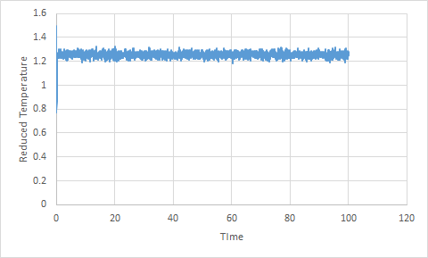
When the timestep is set to be 0.001, the following plots are obtained for the pressure, energy and temperature. It can be seen that all these properties remain constant during the whole simulation.

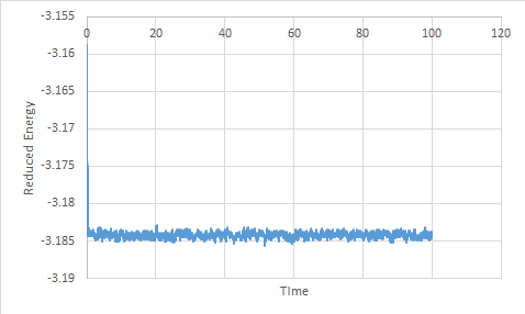
Yes, the simulation reaches equilibrium. It can be seen on Figure 6 that the energy is much higher at the beginning. Once the simulation starts, it decreases significantly very quickly. After that, it remains more or less constant and therefore it's reached equilibrium. It takes 0.3 reduced time units to reach it.

The two timesteps that give the best results are 0.001 and 0.0025, as seen in Figure 7. Sine they both give similar results, we are interested in the one that would take less time to run, this one being 0.0025 as it's a bigger timestep and therefore the same number of steps will cover less actual time than if we used 0.001.
The timestep that gives the worst result is 0.015, when this value is used, the energy does not remain constant and therefore the system doesn't reach equilibrium.
Running Simulations Under Specific Conditions
TASK: We need to choose so that the temperature is correct if we multiply every velocity . We can write two equations:
To obtain a realtionship between and the temperature the equations have to be rearranged. By rearranging the first second one we get:
Since the term also appears in the first equation and is equal to we can rewrite the second equation as follows:
And by cancelling out the terms that are repeated in both sides we get
→
TASK: Use the manual page to find out the importance of the three numbers 100 1000 100000. How often will values of the temperature, etc., be sampled for the average? How many measurements contribute to the average? Looking to the following line, how much time will you simulate?
These values correspond to and respectively and these values tell LAMMPS what timesteps and input values to use to calculate the average of the temperature,etc. Therefore, the temperature,etc. average will be calculated using values that will be sampled every 100 timesteps, 1000 measurements will contribute to the average and an average value will be obtained after 100000 timesteps. Therefore, for this example, we will simulate a total time of 100000.
TASK: When your simulations have finished, download the log files as before. At the end of the log file, LAMMPS will output the values and errors for the pressure, temperature, and density . Use software of your choice to plot the density as a function of temperature for both of the pressures that you simulated. Your graph(s) should include error bars in both the x and y directions. You should also include a line corresponding to the density predicted by the ideal gas law at that pressure. Is your simulated density lower or higher? Justify this. Does the discrepancy increase or decrease with pressure?
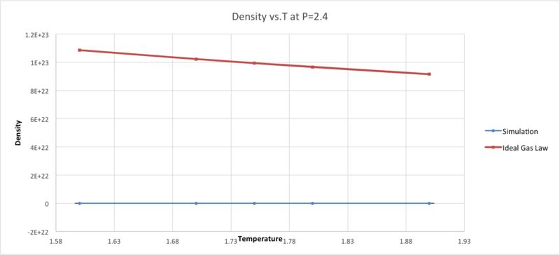
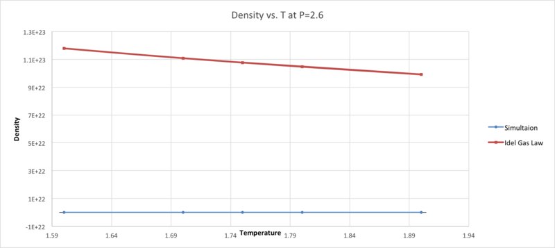
As seen in both graphs, the density predicted by the ideal gas law is higher than the simulated density. This is because the ideal gas law ignores intermolecular interactions and molecular size. Therefore, in this ideal system atoms can get as close to each other as they want since there is no repulsion. In our system, we are not ignoring those interactions so our atoms cannot approach each other as much due to the repulsive forces, decreasing the density of the system with respect to the ideal system. This discrepancy increases with pressure because at higher pressures, the particles are more likely to get closer together and the intermolecular interactions are stronger.
Calculating Heat Capacities Using Statistical Physics
TASK: As in the last section, you need to run simulations at ten phase points. In this section, we will be in density-temperature phase space, rather than pressure-temperature phase space. The two densities required at and , and the temperature range is . Plot as a function of temperature, where is the volume of the simulation cell, for both of your densities (on the same graph). Is the trend the one you would expect? Attach an example of one of your input scripts to your report.

Heat capacity decreases with temperature, as expected, for both densities. At higher densities, it can be seen that the heat capacity is higher. This is because heat capacity is an extensive property and therefore depends on the amount of particles we have. In a given volume, there will be more particles at higher densities than lower densities, meaning that more particles will be able to absorb the heat, making the heat capacity higher.
Example of one of the input scripts:
### DEFINE SIMULATION BOX GEOMETRY ###
lattice sc 0.2
region box block 0 15 0 15 0 15
create_box 1 box
create_atoms 1 box

### DEFINE PHYSICAL PROPERTIES OF ATOMS ###
mass 1 1.0
pair_style lj/cut/opt 3.0
pair_coeff 1 1 1.0 1.0
neighbor 2.0 bin

### SPECIFY THE REQUIRED THERMODYNAMIC STATE ###
variable T equal 2.0
variable timestep equal 0.0025

### ASSIGN ATOMIC VELOCITIES ###
velocity all create ${T} 12345 dist gaussian rot yes mom yes

### SPECIFY ENSEMBLE ###
timestep ${timestep}
fix nve all nve

### THERMODYNAMIC OUTPUT CONTROL ###
thermo_style custom time etotal temp press
thermo 10

### RECORD TRAJECTORY ###
dump traj all custom 1000 output-1 id x y z

### SPECIFY TIMESTEP ###

### RUN SIMULATION TO MELT CRYSTAL ###
run 10000
unfix nve
reset_timestep 0

### BRING SYSTEM TO REQUIRED STATE ###
variable tdamp equal ${timestep}*100
variable pdamp equal ${timestep}*1000
fix nvt all nvt temp ${T} ${T} ${tdamp}
run 10000
reset_timestep 0
unfix nvt
fix nve all nve

### MEASURE SYSTEM STATE ###
thermo_style custom step etotal temp press density
variable dens equal density
variable dens2 equal density*density
variable temp equal temp
variable temp2 equal temp*temp
variable press equal press
variable press2 equal press*press
variable etotal2 equal etotal*etotal
variable etotal equal etotal
fix aves all ave/time 100 1000 100000 v_dens v_temp v_press v_dens2 v_temp2 v_press2 v_etotal2 v_etotal
run 100000

variable avedens equal f_aves[1]
variable avetemp equal f_aves[2]
variable avepress equal f_aves[3]
variable aveetotal equal f_aves[8]
variable avetotal2 equal f_aves[7]
variable heatcapacity equal (((${avetotal2}-${aveetotal}^2)/${avetemp}^2)*atoms^2)/vol

print "Averages"
print "--------"
print "Density: ${avedens}"
print "Temperature: ${avetemp}"
print "Pressure: ${avepress}"
print "HeatCapacity: ${heatcapacity}"
Structural Properties and the Radial Distribution Function
TASK: perform simulations of the Lennard-Jones system in the three phases. When each is complete, download the trajectory and calculate and . Plot the RDFs for the three systems on the same axes, and attach a copy to your report. Discuss qualitatively the differences between the three RDFs, and what this tells you about the structure of the system in each phase. In the solid case, illustrate which lattice sites the first three peaks correspond to. What is the lattice spacing? What is the coordination number for each of the first three peaks?

As seen in Figure 11, there are some differences between the RDFs for a solid, liquid and gas. The RDFs describes how the particles are packed around a reference particle in out system and since the density and the order in the liquid, gas and solid are different, the packing around each atom is expected to be different as well. For all of them, though, it can be seen that at short separations the RDF is 0. This accounts for the effective width of the atoms, as they can't approach any closer.
For a gas, there is a maximum which then rapidly decreases until it reaches one. This peak corresponds to the minimum on the Lennard-Jones potential curve. After that peak, the RDF is pretty much uniform due to the random free motion of the atoms in a gas. For the solid, various peaks are seen which corresponds to the different lattice points where the atoms are located in the crystal structure (fcc in this case). The appearance of long range peaks indicates a higher degree of order in the system, implying a crystal structure. For the liquid, we find some long range order but not as much as in the solid and at higher separation the distribution tends to 1, that is, becomes uniform.
The first three peaks in the solid RDF correspond to the three particles closer to the reference. We know the crystal structure is fcc so by working out the distances between the different lattice point we can find out which one corresponds to which peak. The first three peaks have a separations of 1.025, 1.425 and 1.775.

Figure 12 shows distance a, b and c; a being the smallest one, b the medium one and c the longest one. Therefore,
And assuming a is 1.025, then
Since the second largest distance in the RDF is 1.425 then the atom b corresponds to the second peak and atom a to the first peak.
Similarly, using trigonometry, we can find that which is close enough to the value obtained from the RDF and therefore corresponds to the third peak.
Since the lattice spacing is the same as b,
The coordination number can be obtained by integrating the RDF. The coordination number for the first peak was found to be 12, for the second peak 6 and for the third peak is 12, as expected from a fcc structure.
Dynamical Properties and the Diffusion Coefficient
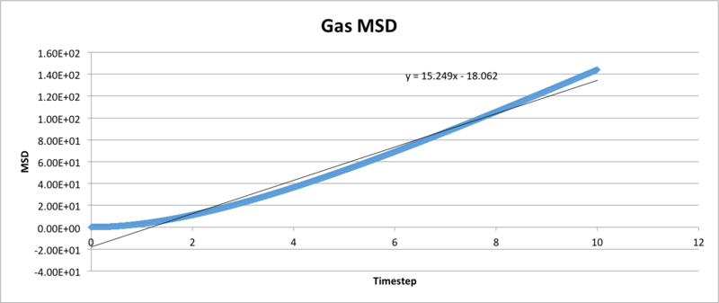
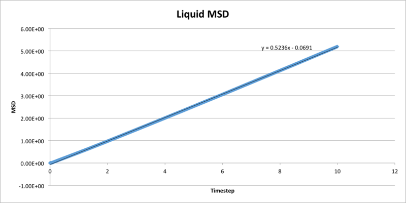
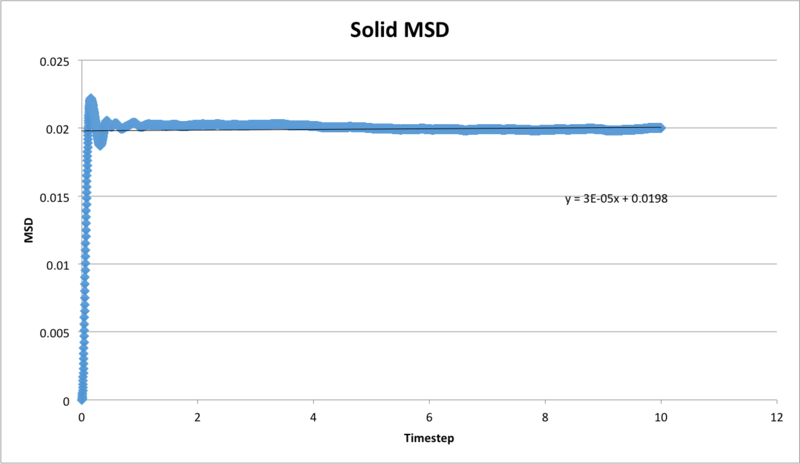
TASK: make a plot for each of your simulations (solid, liquid, and gas), showing the mean squared displacement (the "total" MSD) as a function of timestep. Are these as you would expect? Estimate in each case. Be careful with the units! Repeat this procedure for the MSD data that you were given from the one million atom simulations.
The liquid input file was given. In order to make it appropriate for a gas and a solid, the densities were changed to 0.07 and 1.3 respectively.
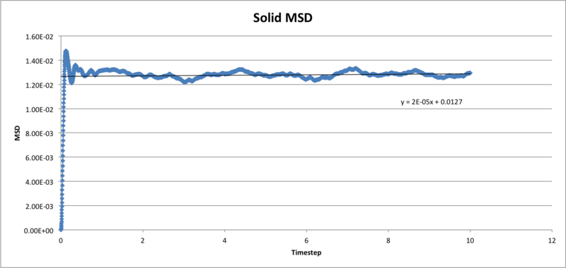

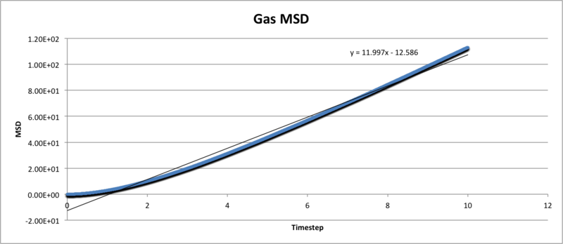
The mean squared distribution measures the spatial extent of random motion of the particles, that is how much of the system a specific particle has visited during the given amount of time. If these values are plotted as a function of time, the graphs seen above are obtained. For the solid, the trend line is almost horizontal, reflecting the lack of movement of the particles in a solid environment. Particles in the liquid and gas phase, however, move more freely and this can be seen by the linear trend of both of these graphs.
The diffusion coefficient, D, is given by the following equation,
We need to find the slope for each function, this is achieved by fitting a linear trend line to each function and extracting the slope from the respective equations. The slope, or , is 11.997 for the gas, 0.5094 for the liquid and 2E-05 for the solid. From that, we can calculate the diffusion coefficient, D, by multiplying each value by 1/6.
The diffusion coefficient is biggest for a gas and smallest for a solid. This makes sense as there is much more freedom of movement in a gas than in a solid where, theoretically, D should be zero. It is not zero because, for this simulation, we're using an approximation.
When plotting the same graphs for a system with one million particles, it was found that the results were really similar. They are particularly similar for the liquid, this is because the density in both systems is the same (i.e. 0.8). However for the other the gas and solid, whilst the density is indeed similar for both the big and small system, they are not exactly the same due to the fact that, in the smaller system, the density was set by me and in the one million particle system the results were given, at an unknown density. Nevertheless, the values are close enough and give really similar results. The slight discrepancy between the small and large system could be due to the fact that the large system represents reality better and therefore will give more accurate results.
The diffusion coefficients for the one million system are the following,
TASK: In the theoretical section at the beginning, the equation for the evolution of the position of a 1D harmonic oscillator as a function of time was given. Using this, evaluate the normalised velocity autocorrelation function for a 1D harmonic oscillator (it is analytic!):
Be sure to show your working in your writeup. On the same graph, with x range 0 to 500, plot with and the VACFs from your liquid and solid simulations. What do the minima in the VACFs for the liquid and solid system represent? Discuss the origin of the differences between the liquid and solid VACFs. The harmonic oscillator VACF is very different to the Lennard Jones solid and liquid. Why is this? Attach a copy of your plot to your writeup.
We first need to find the equation for the velocity for a 1D harmonic oscillator. Since the equation for the position in terms of t is given,, we can differentiate it to get the velocity in terms of t. By doing that we get that the velocity can be described as follows:
Now, we can evaluate both
To make the integration easier, we first rearrange the equations:
Using the following trigonometric identity , the term can be rewritten as follows:
We can now evaluate the integral:
We can take the constants and outside the integral and canceling some terms, we get:
And taking the constants outside the integral:
It can be seen the first term equals to one as the numerator and the denominator are the same. The second term represents a product of odd function and an even function giving an overall odd function (i.e.. It is known that the integral of any odd function will cancel out and equal to zero if the limits set are symmetric across the origin, like in this case. Therefore:
When plotting the VACF and together for a liquid and a solid, it can be seen that there are some differences.
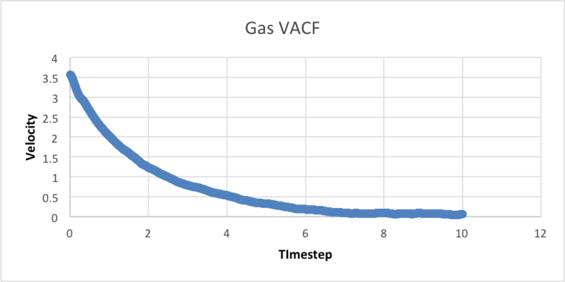

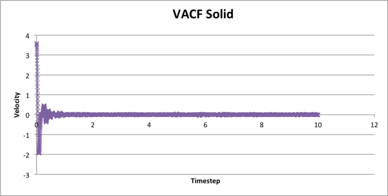

At the beginning the atom will have a specific velocity and if the atoms within the system didn't interact with each other, the atom would always have that same velocity, according to Newton's Laws of motion. Therefore, the plot would just be a horizontal line and so the more horizontal the plot is the weaker the interactions between the atoms.
The minima present in the plot for liquids and solids represent the point where there is a near balance between repulsive forces and attractive forces. This is where the atoms 'want to be' as it's where they are more energetically stable. The atoms in the solid are even more stable in these positions making it hard for them to 'leave' so the atom's motion is an oscillation. These oscillations, though, will decay in time due to interactions with other atoms, which is why we get a plot that looks like a damped harmonic oscillator.
The differences between the liquid and the solid are due to the atoms in the solid being fixed in their lattice points, meaning that they are not free to move around and won't have any movement other than some vibrations. On the other hand, the atoms in the liquid are free to move around and change direction. The minimum in the liquid is less pronounced than in the solid because in the former most of the movement is translational whilst in the latter it's vibrational.
The harmonic oscillator VACF and the Lennard Jones functions look really different because the former assumes a perfect system where there are no forces working against the oscillation of the atoms, so the motion can go on forever.
TASK: Use the trapezium rule to approximate the integral under the velocity autocorrelation function for the solid, liquid, and gas, and use these values to estimate in each case. You should make a plot of the running integral in each case. Are they as you expect? Repeat this procedure for the VACF data that you were given from the one million atom simulations. What do you think is the largest source of error in your estimates of D from the VACF?
To estimate using the trapezium rule approximate we need the following formula:
After using the Trapezium rule to estimate the area under the curve and multiplying each value by 1/3 this is what we get:
For the million particle system:
It can be seen the values for the gas and liquid agree regardless of the method used to calculate them. The values obtained for the gas differ a bit more, probably due to the fact that the graph is not linear so the linear trendline is a worse fit. However, all the values for the gas are really small and close to zero, which is the value we would expect. This shows that both methods are equally accurate at calculating the diffusion coefficient.
The largest source of error when estimating D comes from the inaccuracy of the trapezium rule. The curves we are integrating are not linear and therefore when using the trapezium rule, the results won't be very accurate unless thinner trapezia are used.
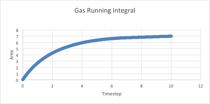


For the million particle system:

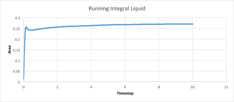
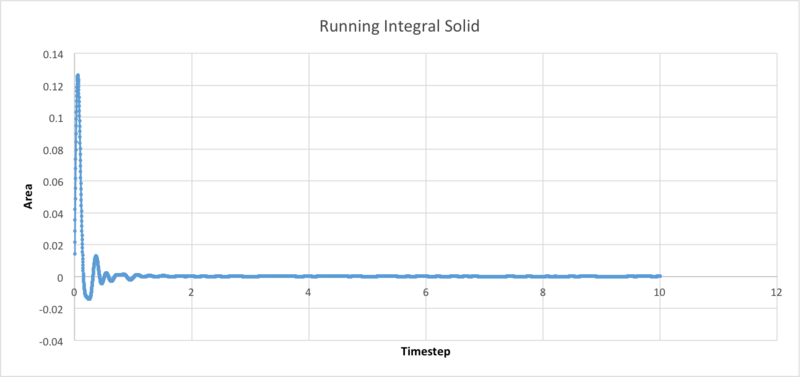
The running integral plots can be seen above, they are all as what we would expect.
