Rep:Mod:3rdyear CMP Exp TPD17

Introduction to the Ising Model

TASK: Show that the lowest possible energy for the Ising model is $E = - D N J$ , where D is the number of dimensions and N is the total number of spins. What is the multiplicity of this state? Calculate its entropy

For a periodic 1D system every spin has 2 possible interactions, 2N interactions, for a periodic 2D system there are 4N interactions, for a 3D system: 6N interaction. From this we can see that there are 2DN interactions for a system of dimension D and size N. However, this counts all the interactions twice so the actual energy is shown by the number of interactions multiplied by the strength of the interaction, J giving the equation $E = - D N J$ . The negative sign is included to

Multiplicity is 2 because the lowest energy system has all spins either up or down

$S = k_{B} l n (2) = 9.57 \times 1 0^{- 24}$

TASK: Imagine that the system is in the lowest energy configuration. To move to a different state, one of the spins must spontaneously change direction ("flip"). What is the change in energy if this happens ( $D = 3, N = 1000$ )? How much entropy does the system gain by doing so?

The energy of the lowest state will be -3000J. The change in energy will be 12J as each of the 6 neighbours to the opposite spin loses one positive interaction and gains a negative one. This means the new energy is -2988J.

the new entropy isː $1.05 \times 1 0^{- 22}$

the gain in entropy is $9.53 \times 1 0^{- 23}$

TASK: Calculate the magnetisation of the 1D and 2D lattices in figure 1. What magnetisation would you expect to observe for an Ising lattice with $D = 3, N = 1000$ at absolute zero?

The magnetisation for both the 1D and 2D lattices is 1. For an Ising lattice $D = 3, N = 1000$ at absolute zero the magnetisation would be 1000 or -1000

Calculating the energy and magnetisation

TASK: complete the functions energy() and magnetisation(), which should return the energy of the lattice and the total magnetisation, respectively. In the energy() function you may assume that J=1.0 at all times (in fact, we are working in reduced units in which J=k_B, but there will be more information about this in later sections). Do not worry about the efficiency of the code at the moment — we will address the speed in a later part of the experiment.

def energy(self):
    "Return the total energy of the current lattice configuration."
    energy = 0.0
    #go through every position in the lattice and calculate the interaction with its neighbours
    for i in range(0,self.n_rows):
        for j in range(0,self.n_cols):
            energy=energy-self.lattice[i,j]*self.lattice[i-1,j]-self.lattice[i,j]*self.lattice[i,j-1]
    return energy

def magnetisation(self):
    "Return the total magnetisation of the current lattice configuration."
    magnetisation = 0.0
    #add up every spin in the lattice
    for i in range(0,self.n_rows):
        for j in range(0,self.n_cols):
            magnetisation=magnetisation+self.lattice[i,j]
    return magnetisation

TASK: Run the ILcheck.py script from the IPython Qt console using the command

 %run ILcheck.py

The displayed window has a series of control buttons in the bottom left, one of which will allow you to export the figure as a PNG image. Save an image of the ILcheck.py output, and include it in your report

As can be seen from the figure, the expected energy and magnetisation of each state was the same as the actual calculated values from my function.

Introduction to Monte Carlo simulation

TASK: How many configurations are available to a system with 100 spins? To evaluate these expressions, we have to calculate the energy and magnetisation for each of these configurations, then perform the sum. Let's be very, very, generous, and say that we can analyse $1 \times 1 0^{9}$ configurations per second with our computer. How long will it take to evaluate a single value of ${⟨ M ⟩}_{T}$ ?

100 spins has 2¹⁰⁰ configurations as each spin can be either up or down. This would take $1.27 \times 1 0^{21}$ seconds which is over 40 trillion years which is way too long for a useful simulation

TASK: Implement a single cycle of the above algorithm in the montecarlocycle(T) function. This function should return the energy of your lattice and the magnetisation at the end of the cycle. You may assume that the energy returned by your energy() function is in units of $k_{B}$ ! Complete the statistics() function. This should return the following quantities whenever it is called: $< E >, < E^{2} >, < M >, < M^{2} >$ , and the number of Monte Carlo steps that have elapsed.

def montecarlostep(self, T):
        "perform a single Monte Carlo step, flip one of the spins in the lattice and determine if it's more favourable"
        #save the initial energy
        energy = self.energy() 
        #update the sums of energy, magnetisation etc
        self.E=self.E+self.energy() 
        self.E2=self.E2+self.energy()**2
        self.M=self.M+self.magnetisation()
        self.M2=self.M2+self.magnetisation()**2
        self.n_cycles=self.n_cycles+1
       
        #the following two lines will select the coordinates of the random spin for you
        random_i = np.random.choice(range(0, self.n_rows))
        random_j = np.random.choice(range(0, self.n_cols))
        #the following line will choose a random number in the range[0,1) for you
        random_number = np.random.random()

       #flip the random spin
        self.lattice[random_i,random_j]=-self.lattice[random_i,random_j]
        #save the final energy
        E1=self.energy()
        #compare energies
        de=E1-energy
        #flip the spin back if it's unfavourable
        if de>0 and random_number>np.exp(-de/T):
            self.lattice[random_i,random_j]=-self.lattice[random_i,random_j]
        return self.energy(), self.magnetisation()

def statistics(self):
        "Calculates the correct values for the averages of E, E*E (E2), M, M*M (M2), number of cycles and returns them"
        #divide sums of properties by the number of cycles
        E=self.E/(self.n_cycles)
        E2=self.E2/(self.n_cycles)
        M=self.M/(self.n_cycles)
        M2=self.M2/(self.n_cycles)
      
        return E,E2,M,M2,self.n_cycles

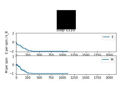
TASK: If $T < T_{C}$ , do you expect a spontaneous magnetisation (i.e. do you expect $⟨ M ⟩ \neq 0$ )? When the state of the simulation appears to stop changing (when you have reached an equilibrium state), use the controls to export the output to PNG and attach this to your report. You should also include the output from your statistics() function.

If $T < T_{C}$ then there will be a spontaneous magnetisation as it is the lowest energy state and the system does not have enough energy to reach equilibrium in a non ordered state^[1].

The ILanim.py file only seemed to run the statistics function for the lattice it generated, not the final Monte Carlo step lattice so all the properties are 0 as this is what they are set to initially before anything is run.

Averaged quantities:
E =  -0.0
E*E =  -0.0
M =  -0.0
M*M =  -0.0

Accelerating the code

TASK: Use the script ILtimetrial.py to record how long your current version of IsingLattice.py takes to perform 2000 Monte Carlo steps. This will vary, depending on what else the computer happens to be doing, so perform repeats and report the error in your average!

6.836964069999988s ± 0.3438758955673139

TASK: Look at the documentation for the NumPy sum function. You should be able to modify your magnetisation() function so that it uses this to evaluate M. The energy is a little trickier. Familiarise yourself with the NumPy roll and multiply functions, and use these to replace your energy double loop (you will need to call roll and multiply twice!).

def energy(self):
        "Return the total energy of the current lattice configuration."
        #create a new lattice rolled 1 position up and one rolled 1 position left
        left=np.roll(self.lattice,1,1)
        up=np.roll(self.lattice,1,0)
        #find interation with original lattice
        one=np.multiply(self.lattice,left)
        two=np.multiply(self.lattice,up)
        #add up interactions
        energy=-np.sum(one+two)
               
        return energy

def magnetisation(self):
        "Return the total magnetisation of the current lattice configuration."
        #add up all the spins
        magnetisation=np.sum(self.lattice)
        return magnetisation

TASK: Use the script ILtimetrial.py to record how long your new version of IsingLattice.py takes to perform 2000 Monte Carlo steps. This will vary, depending on what else the computer happens to be doing, so perform repeats and report the error in your average!

0.27233914545454335s ± 0.006856468109796845

The effect of temperature

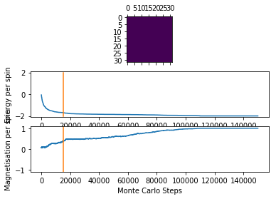
TASK: The script ILfinalframe.py runs for a given number of cycles at a given temperature, then plots a depiction of the final lattice state as well as graphs of the energy and magnetisation as a function of cycle number. This is much quicker than animating every frame! Experiment with different temperature and lattice sizes. How many cycles are typically needed for the system to go from its random starting position to the equilibrium state? Modify your statistics() and montecarlostep() functions so that the first N cycles of the simulation are ignored when calculating the averages. You should state in your report what period you chose to ignore, and include graphs from ILfinalframe.py to illustrate your motivation in choosing this figure.

I chose to start counting after 15000 cycles, because after this number of steps even large lattices like 32x32 have converged to within a reasonable amount of the equilibrium. This large number of steps is perhaps not necessary for smaller lattice sizes, since 32x32 is the largest lattice size the other sizes all converge before it. However after they reach equilibrium their properties don't change very much, so it shouldn't matter greatly how far after convergence the average is taken. Therefore we take all the averages after 15000 cycles.

#set condition so it doesn't collect data before 15000 steps
if self.n_cycles> 15000:
            self.E=self.E+self.energy()
            self.E2=self.E2+self.energy()**2
            self.M=self.M+self.magnetisation()
            self.M2=self.M2+self.magnetisation()**2
#update number of steps
self.n_cycles=self.n_cycles+1

#subtract 15000 from step number or the average will be wrong
E=self.E/(self.n_cycles-15000)
E2=self.E2/(self.n_cycles-15000)
M=self.M/(self.n_cycles-15000)
M2=self.M2/(self.n_cycles-15000)

TASK: Use ILtemperaturerange.py to plot the average energy and magnetisation for each temperature, with error bars, for an $8 \times 8$ lattice. Use your intuition and results from the script ILfinalframe.py to estimate how many cycles each simulation should be. The temperature range 0.25 to 5.0 is sufficient. Use as many temperature points as you feel necessary to illustrate the trend, but do not use a temperature spacing larger than 0.5. The NumPy function savetxt() stores your array of output data on disk — you will need it later. Save the file as 8x8.dat so that you know which lattice size it came from.

As temperature increases so does energy as it is less unfavourable to have opposing spins at higher temperatures. The greater number of opposing spins also creates the trend in the magnetisation graph, where the magnetisation suddenly switches to around 0 after the curie temperature. The error increases with temperature and is especially high around the critical point as it takes longer to equilibrate at higher temperatures.

The effect of system size

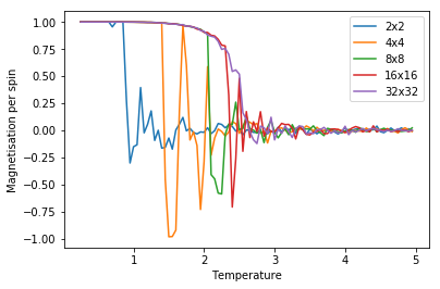
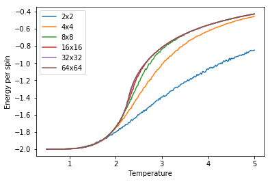
TASK: Repeat the final task of the previous section for the following lattice sizes: 2x2, 4x4, 8x8, 16x16, 32x32. Make sure that you name each datafile that your produce after the corresponding lattice size! Write a Python script to make a plot showing the energy per spin versus temperature for each of your lattice sizes. Hint: the NumPy loadtxt function is the reverse of the savetxt function, and can be used to read your previously saved files into the script. Repeat this for the magnetisation. As before, use the plot controls to save your a PNG image of your plot and attach this to the report. How big a lattice do you think is big enough to capture the long range fluctuations?

The code below is an example of what was done to every file and how all the data was plotted

#load the data file
eight=np.loadtxt('8x8.dat')
#Assign variable names to the data
temp8=eight[:,0]
E8=eight[:,1]
E28=eight[:,2]
M8=eight[:,3]
M28=eight[:,4]
#import matplotlib
from matplotlib import pylab as plt
#plot all the data
plt.plot(temp2,E2/(2*2),label='2x2')
plt.plot(temp4,E4/(4*4),label='4x4')
plt.plot(temp8,E8/(8*8),label='8x8')
plt.plot(temp16,E16/(16*16),label='16x16')
plt.plot(temp32,E32/(32*32),label='32x32')
plt.xlabel('Temperature')
plt.ylabel('Energy per spin')
plt.legend()
plt.show()

In the energy graph it appears that there is little difference in between the 16x16 and the 32x32 suggesting they are big enough to model long range fluctuations. However in the magnetisation graph there still appears to be some difference, so perhaps 32x32 is better to capture long range fluctuations. The periodic nature of this model means that if the lattice size is too small then there will be an interaction between two spins in the same position in neighbouring lattices. In larger lattices this distance is larger so the effect is weaker and we can model the long range fluctuations without the short range interactions getting in the way^[2].

Determining the heat capacity

TASK: By definition,

$C = \frac{\partial ⟨ E ⟩}{\partial T}$

From this, show that

$C = \frac{V a r [E]}{k_{B} T^{2}}$

The definition of variance is the followingː

$V a r [E] = ⟨ E^{2} ⟩ - {⟨ E ⟩}^{2}$

We will need the following definitions to show the heat capacity is equal to $\frac{V a r [E]}{k_{B} T^{2}}$ ː

$β = \frac{1}{k_{B} T}$ (1)

$\frac{\partial β}{\partial T} = \frac{- 1}{k_{B} T^{2}}$ (2)

From statistical thermodynamicsː

${⟨ E ⟩}_{T} = \frac{1}{Z} \sum_{α} E (α) \exp {- β E (α)}$ (3)

${⟨ E^{2} ⟩}_{T} = \frac{1}{Z} \sum_{α} E {(α)}^{2} \exp {- β E (α)}$ (4)

Where Z is the partition function defined asː

$Z = \sum_{α} \exp {- β E (α)}$ (5)

It is useful to take the first and second derivativesː

$\frac{\partial Z}{\partial β} = \sum_{α} - E (α) \exp {- β E (α)}$ (6)

$\frac{\partial^{2} Z}{\partial β^{2}} = \sum_{α} E {(α)}^{2} \exp {- β E (α)}$ (7)

We can substitute equation(6) into equation(3) to get equation(8) and equation(7) into equation(4) to get equation(9)

${⟨ E ⟩}_{T} = \frac{1}{Z} \frac{\partial Z}{\partial β}$ (8)

${⟨ E^{2} ⟩}_{T} = \frac{1}{Z} \frac{\partial^{2} Z}{\partial β^{2}}$ (9)

The definition for heat capacity can be split into two partial derivatives, one of which is defined in equation (2) and can be expressed belowː

$C = \frac{\partial ⟨ E ⟩}{\partial T} = \frac{\partial β}{\partial T} \frac{\partial ⟨ E ⟩}{\partial β} = \frac{- 1}{k_{B} T^{2}} \frac{\partial ⟨ E ⟩}{\partial β}$ (10)

Equation (8) can be substituted into equation (10) to give the following where the chain rule can subsequently be used

$\frac{\partial ⟨ E ⟩}{\partial β} = \frac{\partial}{\partial β} (\frac{- 1}{Z} \frac{\partial Z}{\partial β}) = \frac{\partial \frac{- 1}{Z}}{\partial β} \frac{\partial Z}{\partial β} + \frac{- 1}{Z} \frac{\partial^{2} Z}{\partial β^{2}}$ (11)

$\frac{\partial \frac{- 1}{Z}}{\partial β} = \frac{\partial \frac{- 1}{Z}}{\partial Z} \frac{\partial Z}{\partial β} = \frac{1}{Z^{2}} \frac{\partial Z}{\partial β}$ (12)

Equation (12) can be substituted into equation (11) then subsequently equations (8) and (9) can be substituted in to give something that is the negative definition of variance

$\frac{\partial ⟨ E ⟩}{\partial β} = \frac{1}{Z^{2}} \frac{\partial Z}{\partial β} \frac{\partial Z}{\partial β} - \frac{1}{Z} \frac{\partial^{2} Z}{\partial β^{2}} = {⟨ E ⟩}^{2} - ⟨ E^{2} ⟩ = - V a r [E]$ (13)

If we put equation (13) back into equation (10) the negative signs cancel out and we showː

$C = \frac{V a r [E]}{k_{B} T^{2}}$ (14)

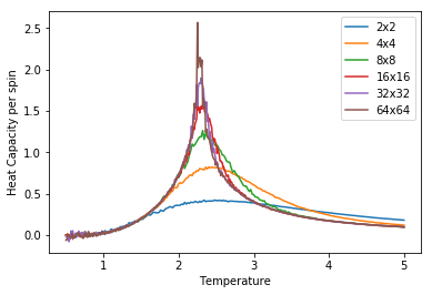
TASK: Write a Python script to make a plot showing the heat capacity versus temperature for each of your lattice sizes from the previous section. You may need to do some research to recall the connection between the variance of a variable, $V a r [X]$ , the mean of its square $⟨ X^{2} ⟩$ , and its squared mean ${⟨ X ⟩}^{2}$ . You may find that the data around the peak is very noisy — this is normal, and is a result of being in the critical region. As before, use the plot controls to save your a PNG image of your plot and attach this to the report.

# the difference of mean of the square of energy with the square of the mean energy, divided by temperature squared
c8=(E28-E8**2)/(temp8**2)

The graph was plotted in the same way as the two plots in the previous section

As lattice size increases so does the size of the peak in the heat capacity. In general the heat capacity increases with temperature until the Curie temperature, when the heat capacity decreases with temperature.

Locating the Curie temperature

TASK: A C++ program has been used to run some much longer simulations than would be possible on the college computers in Python. You can view its source code here if you are interested. Each file contains six columns: $T, E, E^{2}, M, M^{2}, C$ (the final five quantities are per spin), and you can read them with the NumPy loadtxt function as before. For each lattice size, plot the C++ data against your data. For one lattice size, save a PNG of this comparison and add it to your report — add a legend to the graph to label which is which. To do this, you will need to pass the label="..." keyword to the plot function, then call the legend() function of the axis object (documentation here).

The files were loaded in the same way as previously mentioned, and the plots were done in the same way using the relevant data sets

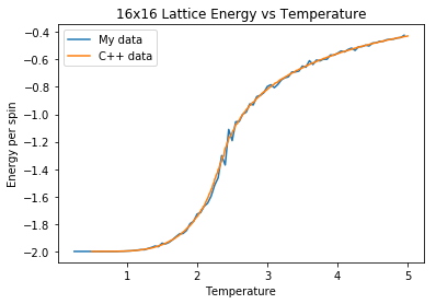
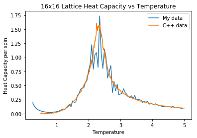
The relative energies, magnetisations and heat capacities with respect to temperature for the different lattice sizes. The same trends are visible as the previously plotted data

In general the C++ data is less noisy than my own generated data. This is likely because the code would be much faster so more steps could be taken for a more reliable average.

TASK: write a script to read the data from a particular file, and plot C vs T, as well as a fitted polynomial. Try changing the degree of the polynomial to improve the fit — in general, it might be difficult to get a good fit! Attach a PNG of an example fit to your report.

#load files
fourc=np.loadtxt('4x4c.dat')
#assign variables
tempc4=fourc[:,0]
Cc4=fourc[:,5]
#create a fit
fit4=np.polyfit(tempc4,Cc4,8)
T_min4 = np.min(tempc4)
T_max4 = np.max(tempc4)
T_range4 = np.linspace(T_min4, T_max4, 1000) 
fitted_C_values4 = np.polyval(fit4, T_range4)
#plot the fit against the data
plt.plot(T_range4, fitted_C_values4)
plt.plot(tempc4,Cc4)
plt.show()

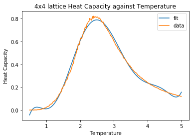
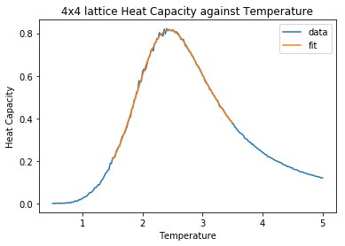
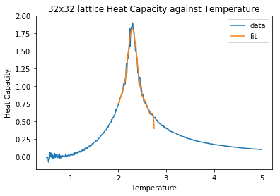
The fit is ok but not great for the lower lattice sizes and in the higher lattice sizes it doesn't really resemble the data at all

TASK: Modify your script from the previous section. You should still plot the whole temperature range, but fit the polynomial only to the peak of the heat capacity! You should find it easier to get a good fit when restricted to this region.

#define the range for the fit
Tmin4=1.5
Tmax4=3.5
s= np.logical_and(tempc4 > Tmin4, tempc4 < Tmax4)
#isolate the data in the range
peak_T=tempc4[s]
peak_C4=Cc4[s]
#create a fit
peakfit4=np.polyfit(peak_T,peak_C4,8)
trange=np.linspace(Tmin4,Tmax4,1000)
fitc4=np.polyval(peakfit4,trange)
#plot the data against the fit
plt.plot(tempc4,Cc4,label='data')
plt.plot(trange,fitc4,label='fit')
plt.xlabel('Temperature')
plt.ylabel('Heat Capacity')
plt.title('4x4 lattice Heat Capacity against Temperature')
plt.legend()
plt.show()

These fits are much better and while not perfect are a much better way of finding the curie temperature as the peak is in the right place.

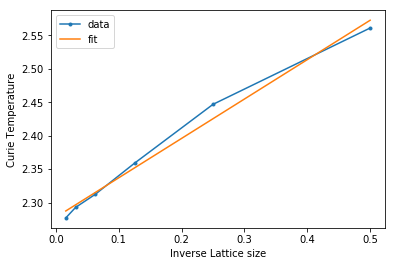
TASK: find the temperature at which the maximum in C occurs for each datafile that you were given. Make a text file containing two columns: the lattice side length (2,4,8, etc.), and the temperature at which C is a maximum. This is your estimate of T_C for that side length. Make a plot that uses the scaling relation given above to determine $T_{C, \infty}$ . By doing a little research online, you should be able to find the theoretical exact Curie temperature for the infinite 2D Ising lattice. How does your value compare to this? Are you surprised by how good/bad the agreement is? Attach a PNG of this final graph to your report, and discuss briefly what you think the major sources of error are in your estimate.

Lattice Side Length	T_C
2	2.56106106
4	2.44694695
8	2.35885886
16	2.31231231
32	2.29279279
64	2.27702703

From the graph, T_c =2.27821603, calculated from the intercept. This compares to T_c = 2.269 in the literature^[3]. This is a reasonably good approximation. The main sources of error will be from all the fits as these are approximations of the data that, as you can see above aren't always perfect. Also, the final linear fit had only 5 points which is not very many, more lattice sizes could be tried out to get a better line to approximate the Curie temperature. More data points in the simulation might help reduce the effect of noise and clean up the heat capacity curve to make the fits more accurate.

References

1. J. Frenkel, J. Doefman, Nature, 1930, 126, 274–275

2. M. Reis, Fundamentals of Magnetism, Elsevier, Amsterdam, 2013, ch.10, 147-175

3. J.Kotze, cond-mat.stat-mech, 2008, https://arxiv.org/pdf/0803.0217.pdf