Third year CMP compulsory experiment

1. Introduction to the Ising model

Task 1:

Show that the lowest possible energy for the Ising model is $E = - D N J$ , where $D$ is the number of dimensions and $N$ is the total number of spins. What is the multiplicity of this state? Calculate its entropy.

The interaction energy is defined as $- \frac{1}{2} J \sum_{i}^{N} \sum_{j \in n e i g h b o u r s (i)} s_{i} s_{j}$ .

By listing out the number of neighbours for each dimension, a relationship can be found.

Dimension	Number of neighbours
1	2
2	4
3	6
$D$	$2 \times D$

For a ground state in the Ising model, all spins would be identical to minimize energy, so $s_{i} = s_{j}$ where $s_{i} = \pm 1$ . Giving $s_{i} s_{j} = 1$ .

Hence:

$- \frac{1}{2} J \sum_{i}^{N} \sum_{j \in n e i g h b o u r s (i)} s_{i} s_{j} = - \frac{1}{2} J \sum_{i}^{N} \sum_{j \in n e i g h b o u r s (i)}$ .

Since the number of neighbours is equal to $2 D$ , $\sum_{j \in n e i g h b o u r s (i)} = 2 D$ .

The lowest possible energy for the Ising model is $E = - \frac{1}{2} J \sum_{i}^{N} (2 D) = - \frac{1}{2} J (N) (2 D) = - D N J$

There are 2 ways for the system to have identical spins, either all are spin up or all or spin down. This gives it a multiplicity of 2. So the entropy of this state is $S = k_{b} \ln 2 = 9.57 \times 1 0^{- 24} J K^{- 1}$

Task 2:

Imagine that the system is in the lowest energy configuration. To move to a different state, one of the spins must spontaneously change direction ("flip"). What is the change in energy if this happens ( $D = 3, N = 1000$ )? How much entropy does the system gain by doing so?

For the single flipped spin $s_{i}$ , spin $s_{i} s_{j} = - 1$ . Then the change in interaction from -1 to 0 to account for the loss of stabilization energy is $\sum_{j \in n e i g h b o u r s (i)} = 2 D (- 1) = - 2 D$ .

The overall change in interaction energy is then $\sum_{j \in n e i g h b o u r s (i)} = 2 D (- 1) + 2 D (- 1) = - 4 D$ to account for the additional gain in destabilization energy.

The spin interaction of the system can be modelled as $\sum_{i}^{N} \sum_{j \in n e i g h b o u r s (i)} = 2 D N + 2 (- 4 D)$ , the destabilization energy is 'subtracted' from the lowest energy state, the factor of 2 accounts for the double counting of the change in interaction. Essentially this also counts the change in interaction in terms of the neighbouring spins which see's the flipped spin, in addition to the change in interaction experienced by the flipped spin itself.

The interaction energy is therefore $- \frac{1}{2} J (2 D N + 2 (- 4 D)) = 4 D J - D N J$ , then:

$Δ E = 4 D J - D N J - (- D N J) = 4 D J$ .

With a dimension of 3, $Δ E = 12 J$ .

The multiplicity for this state is $\frac{1000!}{1! 999!} = 1000$ , this is doubled to account for the opposite spin so $Ω = 2000$ . The entropy for this state is $S = k_{b} \ln 2000$ .

The increase in entropy is $Δ S = k_{b} \ln 2000 - k_{b} \ln 2$

$Δ S = k_{b} \ln \frac{2000}{2}$

$Δ S = k_{b} \ln 1000$

$Δ S = 9.537 \times 1 0^{- 23} J K^{- 1}$

Task 3:

Calculate the magnetisation of the 1D and 2D lattices in figure Fi1. What magnetisation would you expect to observe for an Ising lattice with

D = 3, N = 1000

at absolute zero?

The total magnetisation of the system is given by $M = \sum_{i} s_{i}$

For 1D lattice there are 3 spin ups and 2 spin downs,so:

$M = 3 (1) + 2 (- 1)$

$M = 1$

For the 2D lattice, there are 13 spin ups and 12 spin downs, so:

$M = 13 (1) + 12 (- 1)$

$M = 1$

At absolute zero, the system adopt the lowest energy state where all spins are aligned, hence the magnetisation for an Ising lattice with $D = 3, N = 1000$ would be $M = \pm 1000$

2. Calculating the energy and magnetisation

Task 1:

Complete the functions energy() and magnetisation(), which should return the energy of the lattice and the total magnetisation, respectively. In the energy() function you may assume that $J = 1.0$ at all times (in fact, we are working in reduced units in which $J = k_{B}$ , but there will be more information about this in later sections). Do not worry about the efficiency of the code at the moment — we will address the speed in a later part of the experiment.

Monte carlo simulation:

import numpy as np



class IsingLattice:



    E = 0.0

    E2 = 0.0

    M = 0.0

    M2 = 0.0



    n_cycles = 0



    def __init__(self, n_rows, n_cols):

        self.n_rows = n_rows

        self.n_cols = n_cols

        self.lattice = np.random.choice([-1,1], size=(n_rows, n_cols))



    def energy(self):

        "Return the total energy of the current lattice configuration."

        energy = 0.0
        #For loops loop through every single lattice sight and calculate the energy change due to its neighbors in 2 directions, this avoid double counting. 
        for r in range(0,self.n_rows):

            for c in range(0,self.n_cols):

                energy = energy - (self.lattice[r][c]*self.lattice[r][c-1]) - (self.lattice[r][c]*self.lattice[r-1][c])

        return energy



    def magnetisation(self):

        "Return the total magnetisation of the current lattice configuration."
        #Sums up all of the numbers in lattice sites
        magnetisation = np.sum(self.lattice)

        return magnetisation

Task 2:

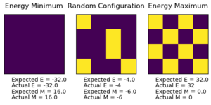
Run the ILcheck.py script from the IPython Qt console using the command

3. Introduction to Monte Carlo simulation

Task 1:

How many configurations are available to a system with 100 spins? To evaluate these expressions, we have to calculate the energy and magnetisation for each of these configurations, then perform the sum. Let's be very, very, generous, and say that we can analyse $1 \times 1 0^{9}$ configurations per second with our computer. How long will it take to evaluate a single value of ${⟨ M ⟩}_{T}$ ?

There are $2^{100}$ configurations in a system with 100 spins. If the analysis speed is $1 \times 1 0^{9}$ configurations per second, then it would take $1.27 \times 1 0^{21}$ seconds to evaluate a single value of ${⟨ M ⟩}_{T}$ , or about 40.2 trillion years! This is about 2900 times longer than the age of the universe!

Task 2:

Implement a single cycle of the above algorithm in the montecarlocycle(T) function. This function should return the energy of your lattice and the magnetisation at the end of the cycle. You may assume that the energy returned by your energy() function is in units of $k_{B}$ ! Complete the statistics() function. This should return the following quantities whenever it is called: $< E >, < E^{2} >, < M >, < M^{2} >$ , and the number of Monte Carlo steps that have elapsed.

    def montecarlostep(self, T):

        # complete this function so that it performs a single Monte Carlo step

        initialenergy = self.energy()

        energyoutput = 0

        #the following two lines will select the coordinates of the random spin for you

        random_i = np.random.choice(range(0, self.n_rows))

        random_j = np.random.choice(range(0, self.n_cols))
        #Flips spin of the chosen lattice site
        self.lattice[random_i][random_j]=-self.lattice[random_i][random_j]
        #Checks the current energy (After spin flip)
        newenergy = self.energy()
        #Calculates difference in energy
        deltaE = newenergy - initialenergy

        


        #the following line will choose a random number in the rang e[0,1) for you

        random_number = np.random.random()
        #Check if energy change is beneficial
        #If energy change not beneficial, it undergoes a probability check where if it passes, the new configuraiton is accepted.
        if deltaE > 0:
 
            if random_number > np.exp(-deltaE/T):
        #If new configuration not accepted, the spin is flipped back and the initial energy before the spin flip is returned.
                self.lattice[random_i][random_j]=-self.lattice[random_i][random_j]

                energyoutput = initialenergy

        else:

            energyoutput = newenergy

                

        
        magnetisationoutput = self.magnetisation()
        #Updates properties of the Ising lattice
        self.E = self.E + energyoutput

        self.E2 = self.E**2 + energyoutput**2

        self.M = self.M + magnetisationoutput

        self.M2 = self.M**2 + magnetisationoutput**2

        self.n_cycles = self.n_cycles + 1

        return (energyoutput,magnetisationoutput)



    def statistics(self):

        # complete this function so that it calculates the correct values for the averages of E, E*E (E2), M, M*M (M2), and returns them

        if self.n_cycles > 0: #prevents division by 0 

            averageE=self.E/self.n_cycles

            averageE2=self.E2/self.n_cycles

            averageM=self.M/self.n_cycles

            averageM2=self.M2/self.n_cycles

        else:

            averageE=self.E

            averageE2=self.E2

            averageM=self.M

            averageM2=self.M2

        return (averageE,averageE2,averageM,averageM2,self.n_cycles)

Averaged quantities: E = -1.519167450611477 E*E = 2453.2692997412983 M = 0.6334960018814676 M*M = 426.60110775076436

Task 3:

If $T < T_{C}$ , do you expect a spontaneous magnetisation (i.e. do you expect $⟨ M ⟩ \neq 0$ )? When the state of the simulation appears to stop changing (when you have reached an equilibrium state), use the controls to export the output to PNG and attach this to your report. You should also include the output from your statistics() function.

The Curie Temperature $T_{C}$ is defined as the transition temperature between a ferromagnetic state of a material to a paramagnetic state. Spontaneous magnetisation decreases as the temperature increases from 0 to $T_{C}$ where spontaneous magnetisation becomes 0.^[2] Below $T_{C}$ , the system will eventually reach a ferromagnetic equilibrium state, this alighment of permanent dipole moments represents an increase in the degreee of order within the system which is associated witha decrease in entropy. This is because at low temperatures the interactions between permanenet dipoles is significant and without sufficient thermal energy to to cause dipoles to point in random directions in zero applied field, the dipoles align themselves as a way to minimize interaction energy, that is to say that the interaction energy stabililzation dominates at low temperatures below $T_{C}$ while above it the effect of entropy dominates as a way to minimize free energy.

Figure 4 - Output of running ILanim.py script

Property	Value
E	-2
E²	4
M	1
M²	1

4. Accelerating the code

Task 1:

Use the script ILtimetrial.py to record how long your current version of IsingLattice.py takes to perform 2000 Monte Carlo steps. This will vary, depending on what else the computer happens to be doing, so perform repeats and report the error in your average!

Time trials for the first version of IsingLattice.py

Trial 1 (s)	Trial 2 (s)	Trial 3 (s)	Trial 4 (s)	Trial 5 (s)	Trial 6 (s)	Average Time (s)	Standard deviation (s)
3.097	3.023	3.058	3.002	2.973	3.155	3.051	0.490

Task 2:

Look at the documentation for the NumPy sum function. You should be able to modify your magnetisation() function so that it uses this to evaluate M. The energy is a little trickier. Familiarise yourself with the NumPy roll and multiply functions, and use these to replace your energy double loop (you will need to call roll and multiply twice!).

import numpy as np



class IsingLattice:



    E = 0.0

    E2 = 0.0

    M = 0.0

    M2 = 0.0



    n_cycles = 0



    def __init__(self, n_rows, n_cols):

        self.n_rows = n_rows

        self.n_cols = n_cols

        self.lattice = np.random.choice([-1,1], size=(n_rows, n_cols))



    def energy(self):

        "Return the total energy of the current lattice configuration."

        energy = 0.0

        energy = - np.sum ( np.multiply ( self.lattice, np.roll( self.lattice, -1, axis = 0))) - np.sum ( np.multiply ( self.lattice, np.roll( self.lattice, -1, axis = 1)))

        return energy



    def magnetisation(self):

        "Return the total magnetisation of the current lattice configuration."

        magnetisation = np.sum(self.lattice)

        return magnetisation



    def montecarlostep(self, T):

        # complete this function so that it performs a single Monte Carlo step

        initial_energy = self.energy()

        magnetisation = self.magnetisation()

        energy_output = 0

        #the following two lines will select the coordinates of the random spin for you

        random_i = np.random.choice(range(0, self.n_rows))

        random_j = np.random.choice(range(0, self.n_cols))

        self.lattice[random_i][random_j]=-self.lattice[random_i][random_j]

        new_energy = self.energy()

        deltaE=new_energy - initial_energy

        


        #the following line will choose a random number in the rang e[0,1) for you

        random_number = np.random.random()

        if deltaE>0:
        #Check if energy change is beneficial
        #If energy change not beneficial, it undergoes a probability check where if it passes, the new configuraiton is accepted.
            if random_number > np.exp(-deltaE/T):

                 self.lattice[random_i][random_j]=-self.lattice[random_i][random_j]

                 energy_output = initial_energy

            else:

                energy_output = new_energy

        else:

            energy_output = new_energy

            


        magnetisation_output = self.magnetisation()

        self.E = self.E + energy_output

        self.E2 = self.E2 + energy_output**2

        self.M = self.M + magnetisation_output

        self.M2 = self.M2 + magnetisation_output**2

        self.n_cycles = self.n_cycles + 1

        return (energy_output, magnetisation_output)



    def statistics(self):

        # complete this function so that it calculates the correct values for the averages of E, E*E (E2), M, M*M (M2), and returns them

        if self.n_cycles > 0:

            averageE=self.E/self.n_cycles

            averageE2=self.E2/self.n_cycles

            averageM=self.M/self.n_cycles

            averageM2=self.M2/self.n_cycles

        else:

            averageE=self.E

            averageE2=self.E2

            averageM=self.M

            averageM2=self.M2

        return (averageE,averageE2,averageM,averageM2,self.n_cycles)

Task 3:

Use the script ILtimetrial.py to record how long your new version of IsingLattice.py takes to perform 2000 Monte Carlo steps. This will vary, depending on what else the computer happens to be doing, so perform repeats and report the error in your average!

Time trials for the second version of IsingLattice.py (Implentation of np.roll and np.sum function)

Trial 1 (s)	Trial 2 (s)	Trial 3 (s)	Trial 4 (s)	Trial 5 (s)	Trial 6 (s)	Average Time (s)	Standard error of the mean (s)
0.228	0.226	0.228	0.223	0.231	0.229	0.228	0.002

Time trials for the third version of IsingLattice.py (Adding the energy and magnetisation values as attributes of the lattice, this prevents repeat calculations in monte carlo steps)

Trial 1 (s)	Trial 2 (s)	Trial 3 (s)	Trial 4 (s)	Trial 5 (s)	Trial 6 (s)	Average Time (s)	Standard error of the mean (s)
0.134	0.133	0.133	0.141	0.139	0.136	0.136	0.003

import numpy as np



class IsingLattice:



    E = 0.0

    Elist = []

    E2 = 0.0

    M = 0.0

    Mlist = []

    M2 = 0.0



    n_cycles = 0

    steps_to_ignore = 3000



    def __init__(self, n_rows, n_cols):

        self.n_rows = n_rows

        self.n_cols = n_cols

        self.lattice = np.random.choice([-1,1], size=(n_rows, n_cols))
        #Stores both energy and magnetisation as a class attribute, this eliminates the need for recalculation in monte carlo step. This allows calling directly from memory and reduce time wasted in          unnecessary calculation
        self.current_energy = self.energy()

        self.current_magnetisation = self.magnetisation()



    def energy(self):

        "Return the total energy of the current lattice configuration."

        energy = 0.0
        #np.roll and np.multiply function is much faster than for loops due to not needing to perform individually calculations for every lattice site
        energy = - np.sum ( np.multiply ( self.lattice, np.roll( self.lattice, -1, axis = 0))) - np.sum ( np.multiply ( self.lattice, np.roll( self.lattice, -1, axis = 1)))

        


        return energy



    def magnetisation(self):

        "Return the total magnetisation of the current lattice configuration."

        magnetisation = np.sum( self.lattice )

        return magnetisation



    def montecarlostep(self, T):

        # complete this function so that it performs a single Monte Carlo step



        #the following two lines will select the coordinates of the random spin for you

        random_i = np.random.choice(range(0, self.n_rows))

        random_j = np.random.choice(range(0, self.n_cols))

        self.lattice[random_i][random_j] = - self.lattice[random_i][random_j]

        

 
        new_energy = self.energy()

        deltaE = new_energy - self.current_energy

        


        if deltaE > 0:

        #the following line will choose a random number in the rang e[0,1) for you

            random_number = np.random.random()        
        #Check if energy change is beneficial
        #If energy change not beneficial, it undergoes a probability check where if it passes, the new configuraiton is acceptoed.
            if random_number > np.exp(-deltaE/T):

                self.lattice[random_i][random_j] = - self.lattice[random_i][random_j]

            else:

                self.current_energy = new_energy

                self.current_magnetisation = self.magnetisation()

        else:

            self.current_energy = new_energy

            self.current_magnetisation = self.magnetisation()



        if self.n_cycles >= self.steps_to_ignore:

            self.E = self.E + self.current_energy

            self.Elist.append(self.current_energy)

            self.E2 = self.E2 + self.current_energy**2

            self.M = self.M + self.current_magnetisation

            self.Mlist.append(self.current_magnetisation)

            self.M2 = self.M2 + self.current_magnetisation**2

    


        self.n_cycles = self.n_cycles + 1

        


        return (self.current_energy, self.current_magnetisation)



    def statistics(self):

        # complete this function so that it calculates the correct values for the averages of E, E*E (E2), M, M*M (M2), and returns them

        if self.n_cycles > 0 and self.steps_to_ignore < self.n_cycles : #prevents division by 0 

            averageE=self.E/(self.n_cycles - self.steps_to_ignore)

            averageE2=self.E2/(self.n_cycles - self.steps_to_ignore)

            averageM=self.M/(self.n_cycles - self.steps_to_ignore)

            averageM2=self.M2/(self.n_cycles - self.steps_to_ignore)

        else:

            averageE=self.E

            averageE2=self.E2

            averageM=self.M

            averageM2=self.M2

        return (averageE,averageE2,averageM,averageM2,self.n_cycles)

5. The effect of temperature

Task 1:

The script ILfinalframe.py runs for a given number of cycles at a given temperature, then plots a depiction of the final lattice state as well as graphs of the energy and magnetisation as a function of cycle number. This is much quicker than animating every frame! Experiment with different temperature and lattice sizes. How many cycles are typically needed for the system to go from its random starting position to the equilibrium state? Modify your statistics() and montecarlostep() functions so that the first N cycles of the simulation are ignored when calculating the averages. You should state in your report what period you chose to ignore, and include graphs from ILfinalframe.py to illustrate your motivation in choosing this figure.

For future investigations, the cut off point for different lattice sizes were determined. The lattice sizes chosen are 2x2, 4x4, 8x8, 16x16, 32x32. Lower temperatures and larger lattices lead to an increase of the number of cycles before the equilibrium state is reached, to minimize the inclusion of these cycles in averages and maintain consistency.

2x2

Temperature	Cutoff point	Cycles
0.1	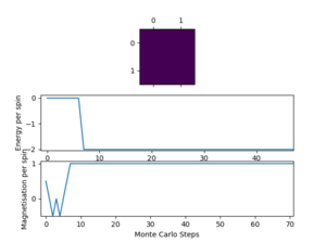10	150000
0.25	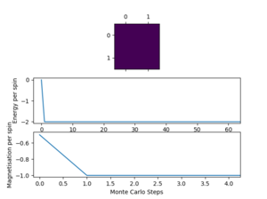5	150000
1	5	150000

4x4

Temperature	Cutoff point	Cycles
0.1	300	15000
0.25	300	15000
1	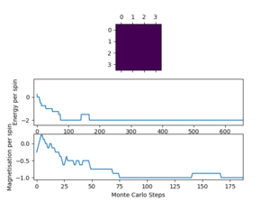300	15000

8x8

Temperature	Cutoff point	Cycles
0.1	1000	15000
0.25	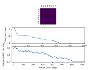1000	15000
1	1000	15000

16x16

Temperature	Cutoff point	Cycles
0.1	10000	30000
0.25	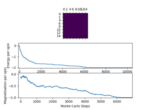10000	30000
1	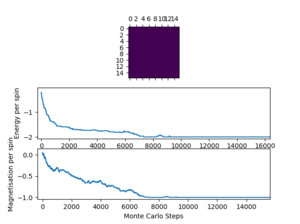10000	30000

32x32

Temperature	Cutoff point	Cycles
0.1	15000	45000
0.25	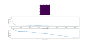15000	45000
1	15000	45000

Task 2:

Use ILtemperaturerange.py to plot the average energy and magnetisation for each temperature, with error bars, for an $8 \times 8$ lattice. Use your intuition and results from the script ILfinalframe.py to estimate how many cycles each simulation should be. The temperature range 0.25 to 5.0 is sufficient. Use as many temperature points as you feel necessary to illustrate the trend, but do not use a temperature spacing larger than 0.5. The NumPy function savetxt() stores your array of output data on disk — you will need it later. Save the file as 8x8.dat so that you know which lattice size it came from.

(Results combined with section 6)

6. Effect of system size

The following graphs show the average magnetisation and energy per spin as temperature increases from 0.25 with error bars.

Figure 4 - Average magnetisation and energy per spin at a temperature range of 0.25 to 5.00 with dT=0.05 for a 2x2 lattice

Figure 5 - Average magnetisation and energy per spin at a temperature range of 0.25 to 5.00 with dT=0.05 for a 4x4 lattice

Figure 6 - Average magnetisation and energy per spin at a temperature range of 0.25 to 5.00 with dT=0.05 for a 8x8 lattice

Figure 7 - Average magnetisation and energy per spin at a temperature range of 0.25 to 5.00 with dT=0.05 for a 16x16 lattice

Figure 8 - Average magnetisation and energy per spin at a temperature range of 0.25 to 5.00 with dT=0.05 for a 32x32 lattice

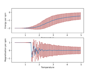
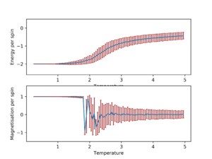
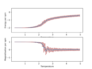
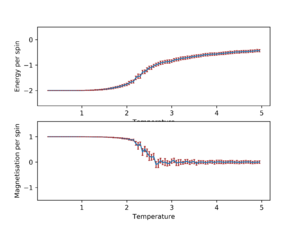
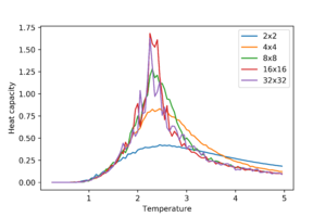
In general, as the lattice size increase, the standard deviation for average energy and magnetisation per spin decreases for all temperatures. The trend appears to stabilize when the lattice size is 16x16 and 32x32 in addition to being very similar to each other, which is more easily seen when they are plotted on the same graph.

Figure 9 - Average magnetisation and energy per spin at a temperature range of 0.25 to 5.00 with dT=0.05 for all size lattices

This would suggest that lattice size of 16x16 or larger should be used in order to capture long range fluctuations.

7. Determining the heat capacity

Task 1:

By definition,

$C = \frac{\partial ⟨ E ⟩}{\partial T}$

From this, show that

$C = \frac{V a r [E]}{k_{B} T^{2}}$

(Where $V a r [E]$ is the variance in $E$ .)

To carry out this differentiation, the product rule was used:

$< E > = \frac{1}{Z} \sum_{α} E (α) e^{- \frac{E (α)}{k_{b} T}}$

Z is the partition function, so:

$\frac{1}{Z} = \frac{1}{\sum_{α} e^{- \frac{E (α)}{k_{b} T}}}$

Using the product rule:

$d (u v) = v d u + u d v$

$\begin{aligned} \frac{d}{d T} (\frac{1}{Z}) = - \frac{1}{{(\sum_{α} e^{- \frac{E (α)}{k_{b} T}})}^{2}} \times \sum_{α} e^{- \frac{E (α)}{k_{b} T}} \times \sum_{α} \frac{E (α)}{k_{b} T^{2}} \\ = - \frac{\sum_{α} E (α) e^{- \frac{E (α)}{k_{b} T}}}{{(\sum_{α} e^{- \frac{E (α)}{k_{b} T}})}^{2} k_{b} T^{2}} \\ = - \frac{1}{Z^{2}} \frac{\sum_{α} E (α) e^{- \frac{E (α)}{k_{b} T}}}{k_{b} T^{2}} \end{aligned}$

$\begin{aligned} \frac{d}{d T} (\sum_{α} E (α) e^{- \frac{E (α)}{k_{b} T}}) = \sum_{α} E (α) e^{- \frac{E (α)}{k_{b} T}} \times \sum_{α} \frac{E (α)}{k_{b} T^{2}} \\ = \frac{\sum_{α} E {(α)}^{2} e^{- \frac{E (α)}{k_{b} T}}}{k_{b} T^{2}} \end{aligned}$

$C = \frac{1}{Z} \frac{d}{d T} (\sum_{α} E (α) e^{- \frac{E (α)}{k_{b} T}}) + \sum_{α} E (α) e^{- \frac{E (α)}{k_{b} T}} \frac{d}{d T} (\frac{1}{Z})$

$\begin{aligned} C = \frac{1}{Z} \times \frac{\sum_{α} E {(α)}^{2} e^{- \frac{E (α)}{k_{b} T}}}{k_{b} T^{2}} + (\sum_{α} E (α) e^{- \frac{E (α)}{k_{b} T}}) (- \frac{1}{Z^{2}} \frac{\sum_{α} E (α) e^{- \frac{E (α)}{k_{b} T}}}{k_{b} T^{2}}) \\ = \frac{1}{Z} \times \frac{\sum_{α} E {(α)}^{2} e^{- \frac{E (α)}{k_{b} T}}}{k_{b} T^{2}} - \frac{1}{Z^{2}} \frac{{(\sum_{α} E (α) e^{- \frac{E (α)}{k_{b} T}})}^{2}}{k_{b} T^{2}} \\ = \frac{< E^{2} > - < E >^{2}}{k_{b} T^{2}} \\ = \frac{V a r [E]}{k_{b} T^{2}} \end{aligned}$

This means that by plotting the heat capacity found with the above equation against temperature, the Curie Temperature can be found at the supposed peaks.

Task 2:

Write a Python script to make a plot showing the heat capacity versus temperature for each of your lattice sizes from the previous section. You may need to do some research to recall the connection between the variance of a variable, $V a r [X]$ , the mean of its square $⟨ X^{2} ⟩$ , and its squared mean ${⟨ X ⟩}^{2}$ . You may find that the data around the peak is very noisy — this is normal, and is a result of being in the critical region. As before, use the plot controls to save your a PNG image of your plot and attach this to the report.

from matplotlib import pylab as pl

import numpy as np

#loads .dat files for each lattice sizes

data2x2=np.loadtxt("2x2.dat")

data4x4=np.loadtxt("4x4.dat")

data8x8=np.loadtxt("8x8.dat")

data16x16=np.loadtxt("16x16.dat")

data32x32=np.loadtxt("32x32.dat")

#Creates list of temperature values

temps=(data2x2[:,0])

#defining a function to return heat capacity values

def C(E,E2,T):

    return (E2-E**2)/(T**2)

C2x2=C(data2x2[:,1],data2x2[:,2],temps)

C4x4=C(data4x4[:,1],data4x4[:,2],temps)

C8x8=C(data8x8[:,1],data8x8[:,2],temps)

C16x16=C(data16x16[:,1],data16x16[:,2],temps)

C32x32=C(data32x32[:,1],data32x32[:,2],temps)

#Plots heat capacity against temperature for all lattice sizes

pl.plot(temps,C2x2/4, label="2x2")

pl.plot(temps,C4x4/16, label="4x4")

pl.plot(temps,C8x8/64, label="8x8")

pl.plot(temps,C16x16/256, label="16x16")

pl.plot(temps,C32x32/1024,label="32x32")

pl.ylabel("Heat capacity")

pl.xlabel("Temperature")

pl.legend()

pl.savefig('heatcap.png',dpi = 600)

pl.savefig('heatcap.svg')

pl.show()

Figure 11 - Temperature vs heat capacity for all lattice sizes using python simulation

8. Locating the Curie Temperature

Task 1:

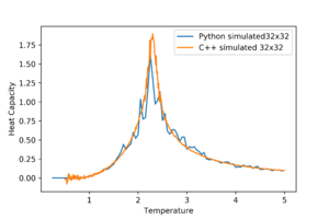
A C++ program has been used to run some much longer simulations than would be possible on the college computers in Python. You can view its source code here if you are interested. Each file contains six columns: $T, E, E^{2}, M, M^{2}, C$ (the final five quantities are per spin), and you can read them with the NumPy loadtxt function as before. For each lattice size, plot the C++ data against your data. For one lattice size, save a PNG of this comparison and add it to your report — add a legend to the graph to label which is which. To do this, you will need to pass the label="..." keyword to the plot function, then call the legend() function of the axis object (documentation here).

Data obtained from C++ simulations are provided and are compared with the data obtained from running python simulations. For the following analysis, the lattice size of 32x32 was used.

Task 2:

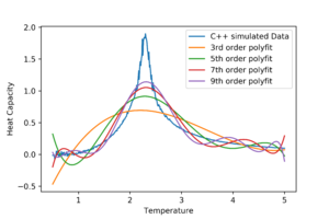
Write a script to read the data from a particular file, and plot C vs T, as well as a fitted polynomial. Try changing the degree of the polynomial to improve the fit — in general, it might be difficult to get a good fit! Attach a PNG of an example fit to your report. To obtain heat capacity and temperature of the peak, polynomials were fitted against the C++ simulated data using the np.polyfit function. A number of different polynomial degrees were used.

from matplotlib import pylab as pl

import numpy as np

#Choosing 32x32 lattice to fit the data, the script would be:

#load c++ data files

cdata32x32=np.loadtxt("C++_data/32x32.dat")

tempsC32x32=(cdata32x32[:,0])

#Get first and sixth column of data for t and c and perform a polyfit over the range of data. Different degrees of polymial fitting attemped below are 3,5,7, and 9

fit3rd32x32=np.polyfit(tempsC32x32, cdata32x32[:,5], 3)

fit5th32x32=np.polyfit(tempsC32x32, cdata32x32[:,5], 5)

fit7th32x32=np.polyfit(tempsC32x32, cdata32x32[:,5], 7)

fit9th32x32=np.polyfit(tempsC32x32, cdata32x32[:,5], 9)



#now we generate interpolated values of the fitted polynomial over the range of our function

T_min = np.min(tempsC32x32)

T_max = np.max(tempsC32x32)

T_range = np.linspace(T_min, T_max, 1000) #generate 1000 evenly spaced points between T_min and T_max

fitted_C_values3rd = np.polyval(fit3rd32x32, T_range) # use the fit object to generate the corresponding values of C

fitted_C_values5th = np.polyval(fit5th32x32, T_range)

fitted_C_values7th = np.polyval(fit7th32x32, T_range)

fitted_C_values9th = np.polyval(fit9th32x32, T_range)

#Plots all polynomialfitting

pl.plot(tempsC32x32,cdata32x32[:,5], label="C++ simulated Data")

pl.plot(T_range,fitted_C_values3rd, label="3rd order polyfit")

pl.plot(T_range,fitted_C_values5th, label="5th order polyfit")

pl.plot(T_range,fitted_C_values7th, label="7th order polyfit")

pl.plot(T_range,fitted_C_values9th, label="9th order polyfit")

pl.xlabel("Temperature")

pl.ylabel("Heat Capacity")

pl.legend()
#save plots
pl.savefig("32x32 lattice polyfits.png", dpi = 600)

pl.savefig("32x32 lattice polyfits.svg")

Task 3:

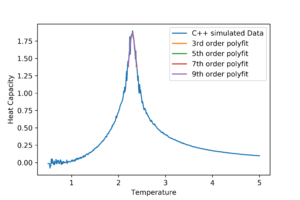
Modify your script from the previous section. You should still plot the whole temperature range, but fit the polynomial only to the peak of the heat capacity! You should find it easier to get a good fit when restricted to this region. As the graph above shows, the higher the order, the better the polynomial is at fitting the data. However none of those still provide a satisfactory fit due to the fitting function attempting to fit across all data points. To solve this the range at which the polyfit function will try to fit is narrowed down as amuch as possible towards the peak present in the data.

from matplotlib import pylab as pl

import numpy as np

#Modifying previous script to only fit near peak

#load c++ data files

cdata32x32=np.loadtxt("C++_data/32x32.dat")

#Tempreatures chosen by visual inspection

Tmin = 2.2

Tmax = 2.4

tempsC32x32=(cdata32x32[:,0])

selection = np.logical_and(tempsC32x32 > Tmin, tempsC32x32 < Tmax) #choose only those rows where both conditions are true





#Get first and sixth column of data for t and c and perform a polyfit over the range of data. Different degrees of polymial fitting attemped below are 3,5,7, and 9

peakfit3rd32x32=np.polyfit(tempsC32x32[selection], cdata32x32[:,5][selection], 3)

peakfit5th32x32=np.polyfit(tempsC32x32[selection], cdata32x32[:,5][selection], 5)

peakfit7th32x32=np.polyfit(tempsC32x32[selection], cdata32x32[:,5][selection], 7)

peakfit9th32x32=np.polyfit(tempsC32x32[selection], cdata32x32[:,5][selection], 9)



#now we generate interpolated values of the fitted polynomial over the range of our function

T_min = np.min(tempsC32x32[selection])

T_max = np.max(tempsC32x32[selection])

T_range = np.linspace(T_min, T_max, 1000) #generate 1000 evenly spaced points between T_min and T_max

peakfitted_C_values3rd = np.polyval(peakfit3rd32x32, T_range) # use the fit object to generate the corresponding values of C

peakfitted_C_values5th = np.polyval(peakfit5th32x32, T_range)

peakfitted_C_values7th = np.polyval(peakfit7th32x32, T_range)

peakfitted_C_values9th = np.polyval(peakfit9th32x32, T_range)

#Plots all polynomialfitting

pl.plot(tempsC32x32,cdata32x32[:,5], label="C++ simulated Data")

pl.plot(T_range,peakfitted_C_values3rd, label="3rd order polyfit")

pl.plot(T_range,peakfitted_C_values5th, label="5th order polyfit")

pl.plot(T_range,peakfitted_C_values7th, label="7th order polyfit")

pl.plot(T_range,peakfitted_C_values9th, label="9th order polyfit")

pl.xlabel("Temperature")

pl.ylabel("Heat Capacity")

pl.legend()
#Save plot
pl.savefig("32x32 lattice peak polyfits.png", dpi = 600)

pl.savefig("32x32 lattice peak polyfits.svg")

Task 4:

Find the temperature at which the maximum in C occurs for each datafile that you were given. Make a text file containing two colums: the lattice side length (2,4,8, etc.), and the temperature at which C is a maximum. This is your estimate of $T_{C}$ for that side length. Make a plot that uses the scaling relation given above to determine $T_{C, \infty}$ . By doing a little research online, you should be able to find the theoretical exact Curie temperature for the infinite 2D Ising lattice. How does your value compare to this? Are you surprised by how good/bad the agreement is? Attach a PNG of this final graph to your report, and discuss briefly what you think the major sources of error are in your estimate.

The curie temperatures for lattice sizes 2x2, 4x4, 8x8 and 16x16 were found similarly and the data was saved as a CurieTemperature.dat file.

from matplotlib import pylab as pl

import numpy as np

#Performing polyfits of 9th order to the rest of the lattice sizes

cdata2x2=np.loadtxt("C++_data/2x2.dat")

cdata4x4=np.loadtxt("C++_data/4x4.dat")

cdata8x8=np.loadtxt("C++_data/8x8.dat")

cdata16x16=np.loadtxt("C++_data/16x16.dat")

cdata32x32=np.loadtxt("C++_data/32x32.dat")

#Setting temperature range to polyfit

Tmin = 2.2

Tmax = 2.4

#Assinging temp range from data to variable

tempsC2x2=(cdata2x2[:,0])

tempsC4x4=(cdata4x4[:,0])

tempsC8x8=(cdata8x8[:,0])

tempsC16x16=(cdata16x16[:,0])

tempsC32x32=(cdata32x32[:,0])

#Assign a chosen t range to a variable

selection2x2 = np.logical_and(tempsC2x2 > Tmin, tempsC2x2 < Tmax)

selection4x4 = np.logical_and(tempsC4x4 > Tmin, tempsC4x4 < Tmax)

selection8x8 = np.logical_and(tempsC8x8 > Tmin, tempsC2x2 < Tmax)

selection16x16 = np.logical_and(tempsC16x16 > Tmin, tempsC16x16 < Tmax)

selection32x32 = np.logical_and(tempsC32x32 > Tmin, tempsC32x32 < Tmax)#choose only those rows where both conditions are true

#Fitting 9th order polynomial to all lattice sizes

peakfit9th32x32=np.polyfit(tempsC32x32[selection32x32], cdata32x32[:,5][selection32x32], 9)

peakfit9th16x16=np.polyfit(tempsC16x16[selection16x16], cdata16x16[:,5][selection16x16], 9)

peakfit9th8x8=np.polyfit(tempsC8x8[selection8x8], cdata8x8[:,5][selection8x8], 9)

peakfit9th4x4=np.polyfit(tempsC4x4[selection4x4], cdata4x4[:,5][selection4x4], 9)

peakfit9th2x2=np.polyfit(tempsC2x2[selection2x2], cdata2x2[:,5][selection2x2], 9)

#now we generate interpolated values of the fitted polynomial over the range of our function

T_min = np.min(tempsC32x32[selection])

T_max = np.max(tempsC32x32[selection])

T_range = np.linspace(T_min, T_max, 1000) #generate 1000 evenly spaced points between T_min and T_max

peakfitted_C_values9th32x32 = np.polyval(peakfit9th32x32, T_range)

peakfitted_C_values9th16x16 = np.polyval(peakfit9th16x16, T_range)

peakfitted_C_values9th8x8 = np.polyval(peakfit9th8x8, T_range)

peakfitted_C_values9th4x4 = np.polyval(peakfit9th4x4, T_range)

peakfitted_C_values9th2x2 = np.polyval(peakfit9th2x2, T_range)

#Extracting Curie Temperature

Cmax2x2=np.max(peakfitted_C_values9th2x2)

Cmax4x4=np.max(peakfitted_C_values9th4x4)

Cmax8x8=np.max(peakfitted_C_values9th8x8)

Cmax16x16=np.max(peakfitted_C_values9th16x16)

Cmax32x32=np.max(peakfitted_C_values9th32x32)



Tmax2x2=T_range[peakfitted_C_values9th2x2==Cmax2x2]

Tmax4x4=T_range[peakfitted_C_values9th4x4==Cmax4x4]

Tmax8x8=T_range[peakfitted_C_values9th8x8==Cmax8x8]

Tmax16x16=T_range[peakfitted_C_values9th16x16==Cmax16x16]

Tmax32x32=T_range[peakfitted_C_values9th32x32==Cmax32x32]



#Saves a .dat file with side lengths and curie temp in 2 columns

np.savetxt("CurieTemperature.dat", np.column_stack(np.array([[2, 4, 8, 16, 32],[Tmax2x2,Tmax4x4,Tmax8x8,Tmax16x16,Tmax32x32]])))

The analysis yielded the following:

Side length	Curie Temperature
2	2.39
4	2.37
8	2.21
16	2.33
32	3.30

The relationship between the Curie temperature and the side length of the square lattice is given as $T_{C, L} = \frac{A}{L} + T_{C, \infty}$ . Using this relationship, the Curie temperature of each lattice size was plotted against the inverse of the sidelength. Then a linear function was fitted against the data. By finding the Y-intercept, $T_{C, \infty}$ can be found.

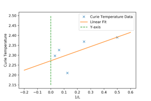
Figure 14 - Plot of inverse of sidelength against Curie Temperature with linear fit

The Y-intercept is given as the last constant term of the polyfit and gives a value of 2.272. The literature equation for the Curie temperature of an infinite 2D square lattice is given as ${T_{C}}^{O n s a g e r} = \frac{2 J}{k_{b} \ln (1 + \sqrt{2})}$ ^[3]. Taking J as 1, ${T_{C}}^{O n s a g e r} = 2.269$ . This represents a difference of 0.088%, which is minimal and is surprisingly in very good agreement with the simulation. The most significant error would have been fluctuations that happened in the simulation.

The following zip file is a jupyter notebook containing scripts used in section 5 - 8. BY1517 2D Ising model.zip

↑ https://wiki.ch.ic.ac.uk/wiki/index.php?title=Third_year_CMP_compulsory_experiment/Introduction_to_the_Ising_model
↑ Hook, J. R., and H. E. Hall. Solid State Physics, John Wiley & Sons, Incorporated, 1991. ProQuest Ebook Central, https://ebookcentral.proquest.com/lib/imperial/detail.action?docID=1212553.
↑ http://www.teori.atom.fysik.su.se/~lindroth/comp08/ising.pdf

[1] ttps://wiki.ch.ic.ac.uk/wiki/index.php?title=Third_year_CMP_compulsory_experiment/Introduction_to_the_Ising_model

[2] Hook, J. R., and H. E. Hall. Solid State Physics, John Wiley & Sons, Incorporated, 1991. ProQuest Ebook Central, https://ebookcentral.proquest.com/lib/imperial/detail.action?docID=1212553.

[3] ttp://www.teori.atom.fysik.su.se/~lindroth/comp08/ising.pdf

[1]

[2]

[3]