Rep:Mod:2580SJ

PART I: Introduction to 3rd Year Computational Labs - Liquid Simulations

The Molecular Dynamics Liquid Simulations lab makes use of the LAMMPS software. In order to simulate a liquid and investigate its properties, numerous ensembles, differing timesteps and algorithms such as the velocity-Verlet are used to conduct analysis. Investigations on the system equilibration, heat capacity, radial distribution function (RDF) and diffusion allow the analysis of the inherent structural properties of a liquid and provide a means for comparing them to a solid and gas.

PART II: Intro to Molecular Dynamics Simulation

Graph 1. Analytical vs. Velocity-Verlet

Graph 2. Total Energy vs. Time

Graph 3 Error vs. Time

VELOCITY VERLET ALGORITHM

By assuming that the acceleration of an atom depends only on its position and not its velocity, it is possible to derive an algorithm that allows calculation of atomic velocities. To use the velocity-Verlet algorithm, it is necessary to know the starting positions of the atoms, x_i(0) and their velocities at that particular time, v_i(0). The velocity-Verlet algorithm can be used to model the behavior of a classical harmonic oscillator.

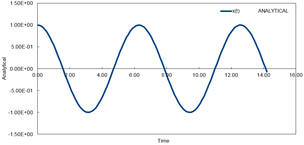
'ANALYTICAL' - contains the value of the classical solution for the position at time t (Graph 1) and is given by:

Classical harmonic oscillator = $A*cos(\omega *t+\varphi )$

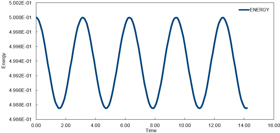
'ENERGY' - contains the total energy of the oscillator for the velocity-Verlet solution (Graph 2) which is given as the sum of kinetic energy and potential energy, using the values for x and v from the velocity-Verlet solution:

E_tot = $\frac{1}{2}m{v}^2+\frac{1}{2}k{x}^2$

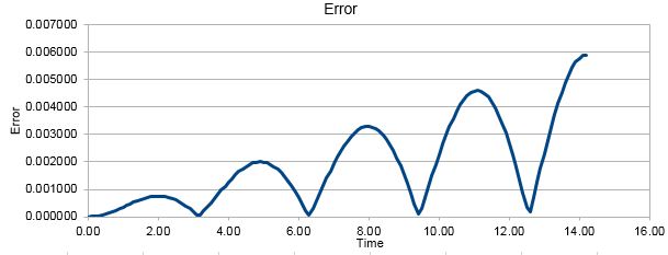
'ERROR' - contains the absolute difference between 'ANALYTICAL' and the velocity-Verlet solution (Graph 3):

Error = $abs[x(t)-ANALYTICAL]$

The following constants are used:

k = 1.0	V(0) = 0.00
Timestep = 0.1000	$\varphi$ = 0.00
Mass = 1.00	A = 1.00
X(0) = 1.00	$\omega$ = 1.00

Graph 4. Error maxima

Error Analysis

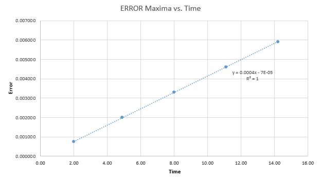
For the default timestep value, 0.1, the positions of the maxima in the ERROR values can be estimated as a function of time. The resulting relation can be seen in Graph 4. This relationship indicates that as the simulation proceeds to longer lengths of time, the errors between the classic solutions and the velocity-Verlet solutions increase linearly.

In order to ensure that the total energy does not change by more than 1% over the course of the simulation, it is necessary to keep the timestep below a value of 0.2. This restriction oversees that the energy oscillates between 0.5 and 0.495 as seen in Graph 5. Timesteps larger than 0.2 will result in a change greater than 1%. It is important to monitor the total energy of a physical system when modelling its behaviour numerically to ensure that the simulation is valid, reasonable and does not lose its physical meaning.

ATOMIC FORCES

It is necessary to make approximations in order to determine the forces acting on a given configuration of atoms. The force that a single atom feels is determined by the position of every other atom in the simulation. In this context, the Lennard-Jones potential can be used to model the interactions between each pair of atoms for many simple liquids, which (for a single interaction) is given by:

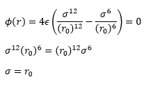
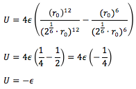
For a single Lennard-Jones interaction, the separation, r₀

 (at which the potential energy is zero) is equal to sigma, σ as seen by the following:

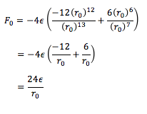
The force, F₀

at this separation is given by the derivative of 

the potential energy with respect to r:

Substituting in r₀ for r and $\sigma$,

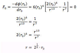
The equilibrium separation, r_eq

is given by:

Since $\sigma =r_0$ and $r=2^{\frac{1}{6}}\cdot r_0$, it follows that the well-depth, ϕ(r_eq)

is given by:

Given that $\sigma =ϵ=1.0$, the integral$\underset{y}{\overset{x}{\int }}\varphi (r)dr$

 using $x=\mathrm{\infty }$ and $y=2\sigma$, $2.5\sigma$, and $3\sigma$, can be solved for. 

With $\mathrm{\infty }$ as a limit, both terms tend towards 0. As a result, the integral gives the following:

PERIODIC BOUNDARY CONDITIONS

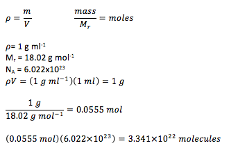
As illustrated below, using realistic volumes of water presents very large numbers of molecules and hence it is not possible to simulate such volumes of liquid.

The number of water molecules in 1 ml of water under standard conditions is given by:

Consider an atom at an initial position (0.5, 0.5, 0.5) in a cubic simulation box, which runs from (0, 0, 0) to (1, 1, 1). When it moves along the vector (0.7, 0.6, 0.2) in a single time step, it ends up at the following position:

Appling the periodic boundary condition gives a set of final position coordinates (0.2, 0.1, 0.7).

REDUCED UNITS

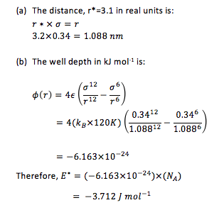
Reduced units (denoted by a star *) are required when using Lennard-Jones interactions to allow for manageable values for calculations. These are calculated by dividing original quantities by scaling factors. This avoids working with values with large negative orders of magnitude. For example,

If the Lennard-Jones parameters for argon are $\sigma =0.34nm$, and $\frac{ϵ}{k_B}=120$, then:

PART III: Equilibration

CREATING THE SIMULATION BOX

In order to start a simulation, the initial states of all the atoms in the system must be known eg. the starting positions. Generating coordinates for atoms in a liquid is challenging, as there is no long-range order. Therefore, it is not possible to use a single point of reference to evaluate the positions of the other atoms, unlike in a solid.

Giving atoms random starting coordinates causes problems in simulations. A random nature implies that there is some probability of atoms being too close together or superimposed on each other, which would result in repulsion and high energy. This would cause inaccuracies errors in the simulation process and generation of valid results would be difficult. Instead, a model of a simple cubic lattice will be used. Even though this is not a realistic representation of the physical state, it is found that if the simulation is prolonged for a certain amount of time, the atoms rearrange themselves into more realistic configurations.

Lattice sc 0.8 Lattice spacing in x,y,z = 1.07722 1.07722 1.07722

The first command in the input file creates a grid of points forming a simple cubic (sc) lattice. The parameter 0.8 specifies the number density, which is given by:

The second line in the output file indicates the distance between lattice points in reduced units. A simple cubic lattice consists of one lattice point in total. Therefore, lattice spacings of 1.07722 correspond to a number density of 0.8 as follows:

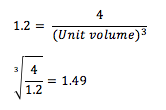
The face-centred cubic (fcc) lattice consists of four lattice points in total. If the number density is 1.2, the side length of the cubic unit cell can be calculated to be 1.49 as follows:

In addition, since the fcc lattice as four lattice points and hence atoms, it can be defined as having three more atoms compared to a simple cubic. Therefore, since there are 1,000 atoms for the simple cubic, there should be 1,000 + (3 x 1,000) = 4,000 atoms.

SETTING PROPERTIES OF THE ATOMS

The following commands in the input script are defined and explained below:

mass 1 1.0 = sets the mass for all atoms of type 1 to mass 1.0

pair_style lj/cut 3.0 = computes the standard 12/6 LJ potential; sets the formula to compute pairwise interactions (pair potentials are defined between pairs of atoms that are within a certain cut-off distance) with a LJ cut-off = 3.0

pair_coeff * * 1.0 1.0 = specifies the pairwise force field coefficients for one or more pairs of atom types; explicit numeric values can be specified for the atom types, in this case, all atoms 1 through N are assigned 1.0

Given that x_i(0) and v_i(0) are specified, the integration algorithm which will be employed is the velociy-Verlet algorithm, as explained previously.

RUNNING THE SIMULATION

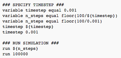
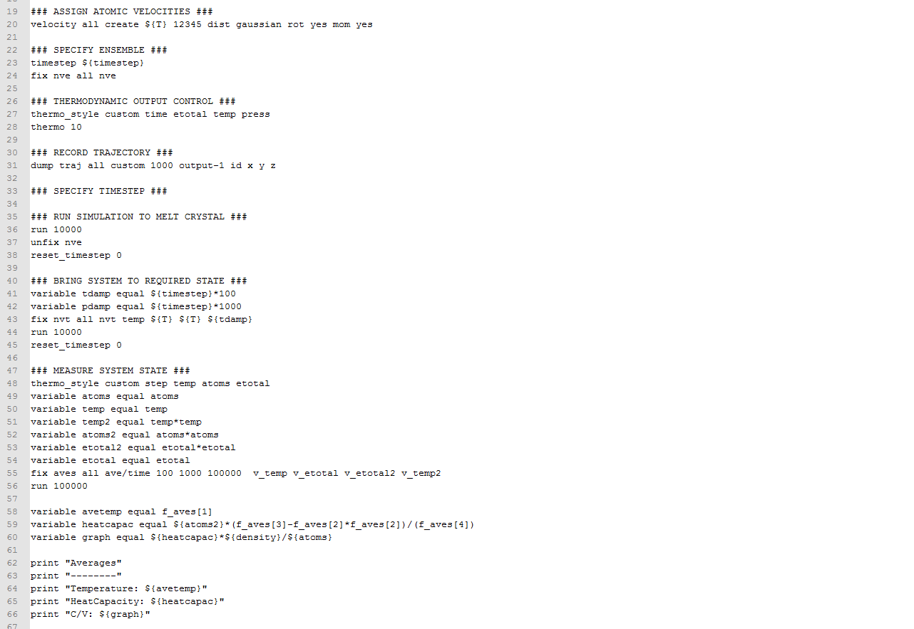
The above code is used in order to allow the variable to be defined once, so that everything that is dependent on that particular variable will change values accordingly. The code permits the variable to be re-used. If the simulation were to be run again at different conditions, it would merely be a case of changing the value of the particular variable at the beginning of the script as opposed to every section where it applies. This method circumvents repetitive manual inputting.

CHECKING EQUILIBRATION

Graph 5. Total energy, temp, pressure vs. Time (time step=0.001)

Graph 6. Total energy vs. Time for various time steps

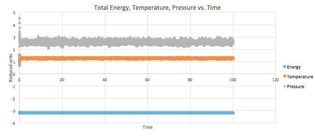
Total energy, temperature and pressure can be plotted in reduced units as a function of time (time step = 0.001) as seen in Graph 5.

The simulation reaches equilibrium as the values for pressure, energy and temperature level off at a certain point of time, however, there are constant fluctuations around an average value. If the graphs are zoomed in, it is possible to see that the plateau starts at 0.3 and hence this is how long it takes the system to reach equilibrium.

In order to choose a timestep effectively, it is necessary to balance out and compromise between the accuracy, physical meaning and time needed to acquire the information.

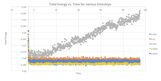
As seen in Graph 6, The simulation with time step = 0.015 is not a good choice of timestep because the system does not reach equilibrium as seen by the plot of energy against time. Instead, the values increase with increasing time.

0.001 is the smallest timestep and hence will provide the most accurate depiction of physical reality through the simulation. However, this also means that the same number of simulation steps cover a relatively shorter amount of actual time. Therefore, if a process that requires long observation time is to be analysed, this timestep would be ineffective. 0.0025 is the second smallest timestep and has similar results as 0.001.

As the timestep becomes larger than 0.0075, the values obtained start to deviate.

Hence, the best choice for a reasonable timestep is 0.0025.

PART IV: Running Simulations Under Specific Conditions

THERMOSTATS AND BAROSTATS

Contrasting to the previous section, the simulations are now going to be run under NpT conditions as opposed to NVE. A sketch of an equation of state for the model fluid at atmospheric pressure will be made under NpT conditions. 5 temperatures (above the critical temperature of T*=1.5) were chosen and 2 pressures (using the average pressure from the previous simulation) were chosen to generate ten phase points as seen in Table 1. Each simulation was run for each chosen (p, T). The timestep = 0.0025.

Table 1. NpT Conditions

Run	P*, T*	Run	P*, T*
1	2.3, 2.0	2	2.7, 2.0
3	2.3, 3.0	4	2.7, 3.0
5	2.3, 4.0	6	2.7, 4.0
7	2.3, 4.5	8	2.7, 4.5
9	2.3, 5.0	10	2.7, 5.0

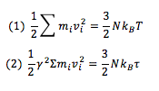
The equipiartition theorem states that, on average, every degree of freedome ina system at equilibrium will have $\frac{1}{2}{k}_{B}T$ of energy. In the present system with N atoms, each with three degrees of freedom, the following can be expressed:

The instantaneous temperature, T, is obtained by using the above equation. However, in general, T will fluctuate and will essentially be different to the target temperature, $\tau$ (the input value). It is possible to change the temperature by multiplying every velocity by a constant factor, $\gamma$.

If T> $\gamma$, then the KE of the system is too high and needs to be reduced ($\gamma <1$).

If T> $\gamma$, then the KE of the system is too low and needs to be increased ($\gamma >1$).

The constant factor, $\gamma$ needs to be chosen so that T= $\tau$. Therefore, in order to solve for γ, the following two equations can be written and solved simultaneously:

By subtracting (1) from (2) and letting Σm_i v_i^2=S,

Substituting in the expanded form of S,

EXAMINING THE INPUT SCRIPT

In the input script, the below instructs LAMMPS to ‘bring the system to a required state’. Average thermodynamic properties for the system can be measured by detailing specific commands. In order to draw the equations of state, the average temperature, pressure, density and statistical erros in the respective quantities need to be known. The averaging command is in the line starting with ‘fix aves…’:

The three numbers 100, 1000, 100000 indicate N_every, N_repeat, and N_ferq. This command tells LAMMPS to use the input value after every 100 timesteps ( N_every) so that a total of 1,000 timesteps (N_repeat) have been used to calculate the average after 100,000 timesteps (N_ferq).

PLOTTING THE EQUATIONS OF STATE

Graph 7. Average density vs. Time (P*=2.3)

Graph 8. Average density vs. Time (P*=2.3)

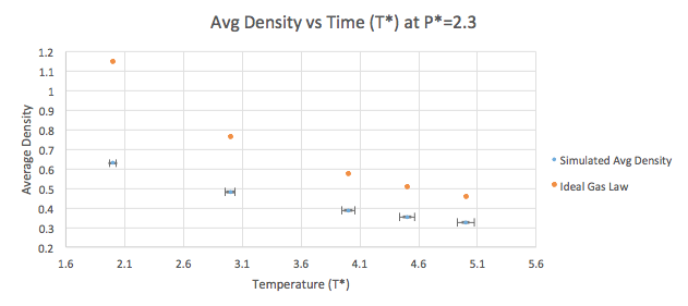
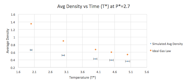
The density can be plotted as a function of temperature (Graphs 7-8) for both of the pressures that were simulated as listed in Table 2. A line corresponding to the density predicted by the Ideal Gas Law (pV=nRT) is plotted for both the pressure values. The simulated density is clearly lower than that predicted by the Ideal Gas Law. This can be explained by the assumptions the Law stands on. According to the Law, density is proportional to the temperature (at constant pressure). In an ideal gas, all interactions (both attractive and repulsive) are ignored, which is not the case in the simulation. This means that the density at a given point will seem higher than what it actually is as the atoms are not repelling each other. The difference between the Ideal Gas Law and the LAMMPS simulation increases at higher pressure values. This arises from the fact that at constant temperature, the density is proportional to the pressure.

PART V: Calculating Heat Capacities Using Statistical Physics

In statistical thermodynamics, many quantities can be calculating by considering how far the system is able to fluctuate from its average equilibrium state. For example, under conditions of constant temperature, the total energy fluctuates. The magnitude of these fluctuations gives information of the system’s heat capacity:

Graph 9. Heat capacity vs. Temp (density=2.3, 2.7)

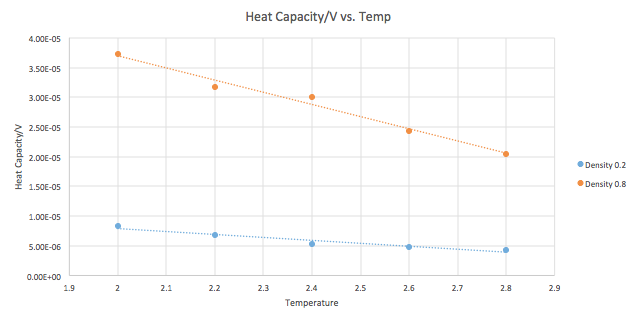
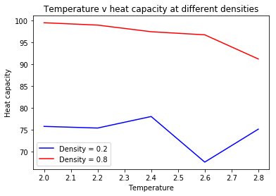
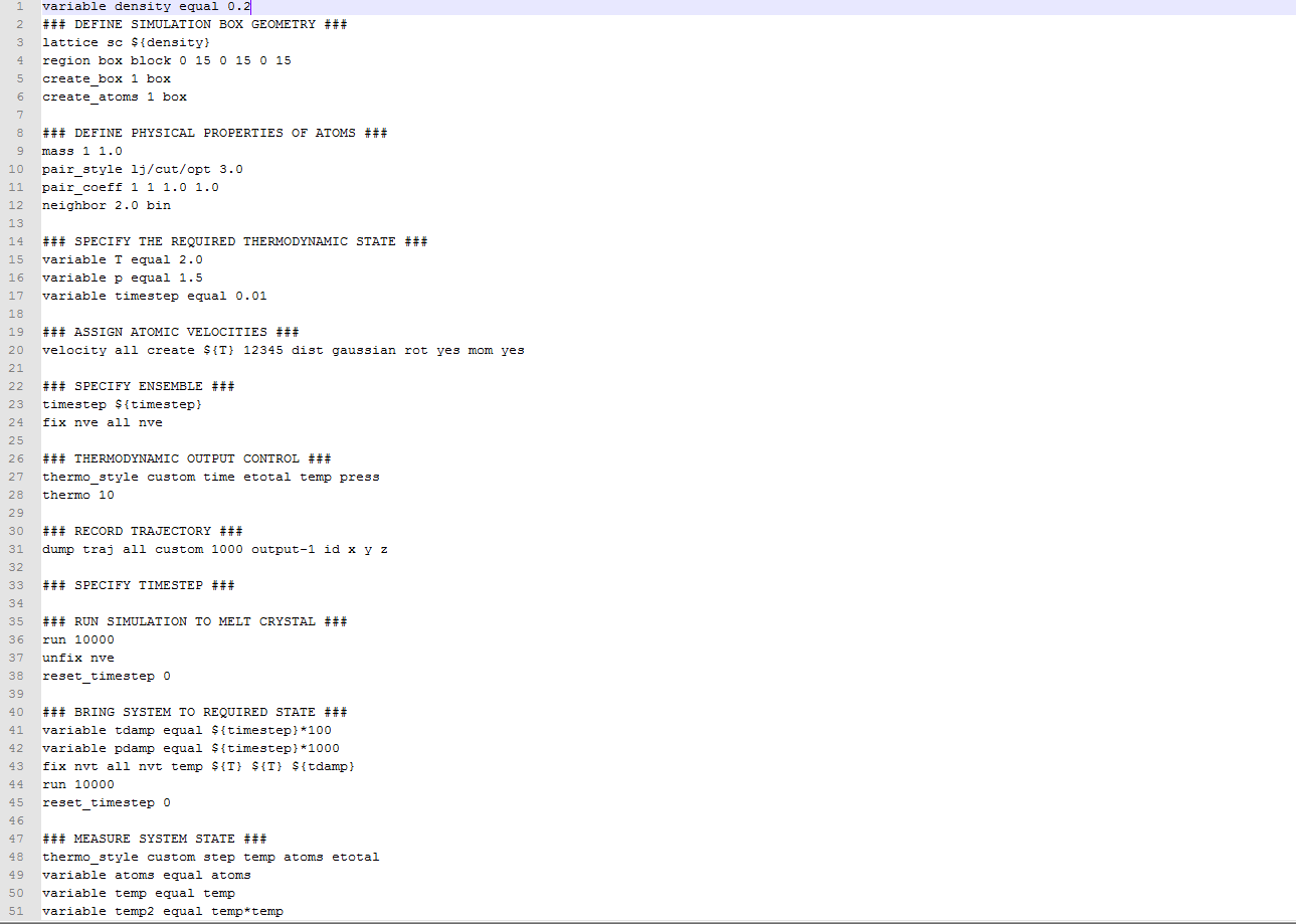
Once again, simulations were run at ten phase points. The difference is that the system is now in a density-temperature (ρ*, T*) phase space as opposed to a pressure-temperature phase space. The values used for both are indicated in Table 2. An example of the input script can be seen below. The output results were used to plot CV/V as a function of temperature for both the densities (Graph 9).

Run	$\rho$*, T*	Run	$\rho$*, T*
1	0.2, 2.0	2	0.8, 2.0
3	0.2, 2.2	4	0.8, 2.2
5	0.2, 2.4	6	0.8, 2.4
7	0.2, 2.6	8	0.8, 2.6
9	0.2, 2.8	10	0.8, 2.8

Heat capacity is the energy a substance requires to raise the temperature of the system by 1 degree. The general trend indicates that as the density increases, the heat capacity increases, across all temperatures. An increase in density means an increase in the number of atoms in a fixed volume. Consequently, the system requires a larger amount of energy to raise the temperature by 1 degree, as each of the atoms need to be raised in energy to achieve this.

The graph indicates that as the temperature increases, the heat capacity of the system decreases. At higher temperatures, the system already has a certain amount of energy, higher than the original state at the original temperature. As a result, the energy levels (vibrational, rotational, and translational) are closer together and the system requires less energy as a whole to raise the temperature. There is also greater probability of finding high energy levels.

The probability of finding particles in these energy levels increases as a consequence of both increasing density and temperature. Due to this, the system requires less energy to impart to its particles in order to raise the temperature by 1 degree. The energy of the system is closer to the amount of energy that is required to achieve this state. This accounts for the steeper slope seen in the plot for density=0.8 compared to density=0.2.

PART VI: Structural Properties and the Radial Distribution Function (RDF)

Figure 1. Leannard-Jones system phase diagram

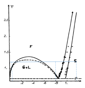
The structure of the systems that are simulated can be characterized by RDF’s. These are denoted by g(r) and is an indication of the distances from an atom at which its neighbors can be found. VMD is used to calculate the RDF for the solid, liquid, and vapor phases of the Lennard-Jones fluid using the following conditions (found through analyzing the phase diagram in Figure 1):

Graph 10. RDF for a solid, liquid and gas

Figure 2. FCC lattice nearest neighbors

Graph 11. RDF g(r) integral for a solid, liquid and gas

- Liquid = T(1.2), $\rho$(0.8)

- Gas = T(1.2), $\rho$(0.05)

- Solid = T(1.2), $\rho$(1.2)

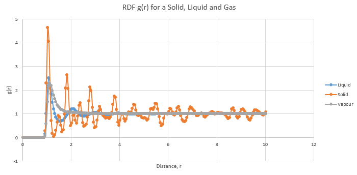
The radial distribution function (RDF) is used to find information about the structure of the system by describing the variation in the probability of finding particles as a function of time. In Graph 10, the differences between the RDFs of a solid, liquid and gas are apparent.

In a gas, although there is a high probability of finding the first neighbor, closest to the reference atom, this probability plummets significantly as the distance increases. They physical significance of this is that since the atoms or molecules in a gas are far apart and randomly dispersed, the probability of finding another atom is very low. A liquid has more long-range order and therefore displays multiple peaks in the RDF, three of them which are well-defined. This is a consequence of liquids having a somewhat structured environment around the one atom for example, the primary and secondary solvation shells. The solid RDF has numerous well-defined peaks which owe to its fixed structure and hence well-defined neighbors. All the graphs eventually level off to a value of 1. At this point, it is implied that the density of all the phases at local points is fairly constant.

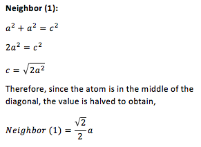
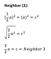
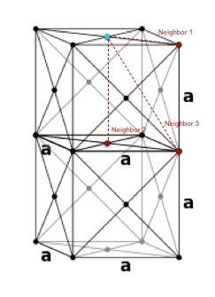
Since the peaks indicate the distance of the nearest neighbors relative to the reference atom, it is possible to find the positions of the nearest neighbors in a solid structure. The first, second and third peaks correspond to the first, second and third neighbors, respectively. Using trigonometry it is possible to calculate the positions of these neighbors in an fcc lattice. On Fig. 2, the reference atom is given in blue while the first three neighbors are given in red. Hence, the lattice sites that the first three peaks in the solid RDF correspond to are as follows:

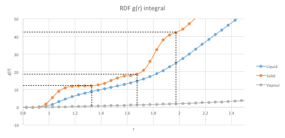
The average coordination numbers for each of the three peaks can be found by analyzing the RDF g(r) integral in Graph 11. The RDF for each peak is integrated to the the minima corresponding to each peak. This is denoted by the end of each plateau. The values of the integral are read off the graph and are found to be as below. Note that since it is a cumulative function, the previous values need to be subtracted from the considered value in order to obtain the coordination number (CN).

Neighbor 1 CN = 12

Neighbor 2 CN = 18-2=6

Neighbor 3 CN = 42-18=24

PART VII: Dynamical Properties and Diffusion Coefficient

Graph 12. Total MSD for a solid (small system)

Graph 13. Total MSD for a liquid (small system)

Graph 14. Total MSD for a vapour (small system)

Graph 15. Total MSD for a solid (large system)

Graph 16. Total MSD for a liquid (large system)

Graph 17. Total MSD for a vapour (large system)

MEAN SQUARED DISPLACEMENT (MSD)

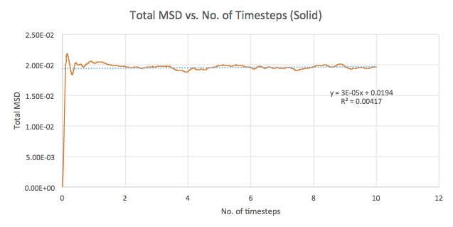
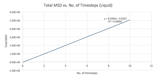
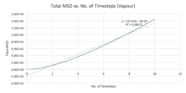
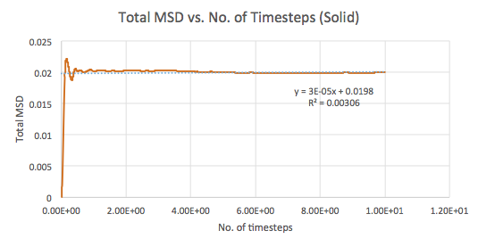
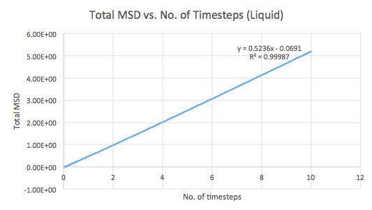
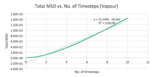
The mean squared displacement (MSD) is used as a measure of spatial extent of random motion. Graphs 12-14 of total MSD versus timestep are plotted for a solid, liquid and gas. By using a linear best fit, the slope can be used to estimate the value of the diffusion coefficient, D as follows:

Small system:

Phase	Slope	Diffusion coefficient (D)
Solid	0.00003	0.000005
Liquid	0.5094	0.0849
Gas	15.216	2.536

Large system:

Phase	Slope	Diffusion coefficient (D)
Solid	0.00003	0.000005
Liquid	0.5236	0.0873
Gas	15.249	2.542

The values of D are as expected in the order gas > liquid > solid. Gases displays the largest D as the system has the greatest ability to diffuse its atoms as a result of the random, spread out nature and tendency for the atoms to move around freely and quickly. Liquids also exhibit a certain level of diffusion. However, solids have little to no diffusion due to their rigid and ordered structure, explaining the extremely small value for D. Comparing the values for the small and large systems (Graphs 15-17), it can be seen that there is slight difference between the liquid and gas. The latter values should be more representative for a realistic system as the model is much larger. The discrepancies between the small and large systems may arise due to the errors while running the simulation.

VELOCITY AUTOCORRELATION FUNCTION (VACF)

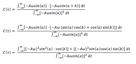
Alternatively, the diffusion coefficient can be calculated using the velocity autocorrelation function which is given by:

The VACF is a time-dependent correlation function. For every atom in the system, three components of the velocity are stored for each Cartesian coordinate. The function indicates how different the velocity of an atom will be at time t + $\tau$ to its velocity at time t. At long times, C $(\mathrm{\infty })$ = 0 because the velocities of atoms become ‘uncorrelated’ at long times. By integrating the following function, the diffusion coefficient can be found:

The normalized velocity autocorrelation function for a 1D harmonic oscillator is:

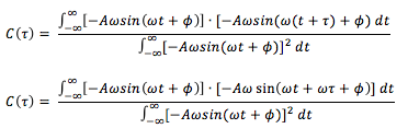
The equation for the evolution of the position of a 1D harmonic oscillator as a function of time (introduced previously) can be used to evaluate the normalized velocity autocorrelation function (VACF) as follows:

Classical harmonic oscillator = $A*cos(\omega *t+\varphi )$

Since the derivative of position with respect to time is velocity,

The above derivative can be substituted into the equation for $C(\tau )$:

Using the trigonometry identity, $sin(a+b)=sin(a)cos(b)+cos(a)sin(b)$ and letting $a=\omega t+\varphi$ and $b=\omega \tau$, the above can be further simplified:

The fraction can be separated into two separate fractions and since $A\omega$ and $b=\omega \tau$ are constants, these terms can be taken outside the integral. This allows further simplification:

Since $sin(a)cos(a)$ are odd and even functions, when these are integrated using symmetric limits, the integral goes to 0. Therefore, the integral term on the RHS becomes 0, leaving:

Graph 18. Harmonic oscillator compared to simulated solid and liquid system VACFs

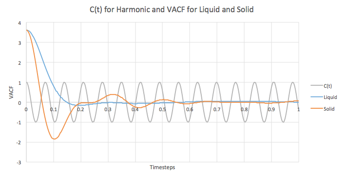
Graph 18 is a plot of C $(\tau )$ and also the VACF’s from the liquid and solid simulations that were run. The equation illustrates the decay of the correlation in the two specific systems being modelled. The difference between the VACF graphs for the solid and liquid arise from the difference in system order and structure. A solid displays regular order with atoms closely packed together in a way that balances out repulsive and attractive forces. This favorable balance means that atoms prefer to stay in such configurations and cannot easily be removed from them. As a result, the motion of the atoms is just an oscillation and the VACF reflects this. However, the oscillations are not perfect, but are unequal in magnitude and eventually decay to level off. In the case of liquids, the atoms no longer have fixed positions. Although there is an initial correlation as seen by the clear oscillation, diffusion interferes with the oscillatory motion and therefore, the VACF rapidly decays to 0. The minima in the solid and liquid graphs indicate the largest and maximum velocity achieved by the oscillatory motion of the atoms in the respective systems.

The large discrepancy between the graph for the harmonic oscillator compared to the Lennard Jones solid and liquid can be explained by the fact that the former disregards any forces that may perturb or act against the oscillations.

Graph 19. Integrals for small and large systems using trap rule (solid)

Graph 20. Integrals for small and large systems using trap rule (liquid)

Graph 21. Integrals for small and large systems using trap rule (vapor)

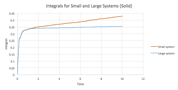
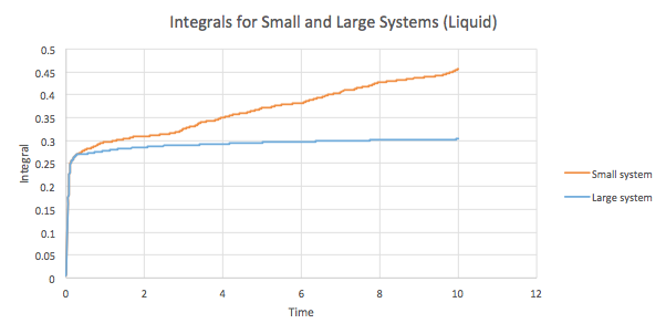
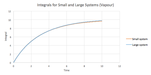
The trapezium rule can be used to approximate the integral under the VACF graphs for the solid, liquid and gas as seen in Graphs 19-21. Using these values, a value for D can be found as well.

Small system:

Phase	Integral	Diffusion coefficient (D)
Solid	0.427985851	0.14266195
Liquid	0.455802947	0.151934316
Gas	9.67334816	3.224449387

Large system:

Phase	Integral	Diffusion coefficient (D)
Solid	0.353838221	0.117946074
Liquid	0.303172884	0.101057628
Gas	0.133213000	3.268465798

Error analysis

The results obtained by plotting the integrals are as expected. The general trend indicates that the diffusion coefficient increases as the system disorder increases, gas > liquid > solid. However, as the time increases, the integral values for the solid and liquid phases in the small and large systems deviate to a larger extent, from one another. In addition, there is a slight anomalous result in the D values for the large system. The solid has a slightly higher D than the liquid which does deviates from the trend predicted and observed in the other results. This is most probably a result of errors while estimating the diffusion coefficient. The trapezium integral method is used to estimate the integrals and since this is an approximation, the values obtained are not the most accurate. In addition, the rule depends on the timestep and hence the accuracy is limited to this. As a result, the use of this method stands as the largest source of error in the calculation of D.