
Rep:Mod3GL1990
Module 3 - George Lane
Cope Rearrangement
Introduction

A Cope rearrangement is a widely studied [3,3] sigmatropic rearrangement reaction of 1,5 dienes. The reaction is a pericyclic reaction where one sigma bond is broken and one sigma bond is formed from a concerted aromatic transition state, it wasdiscoverd in 1940 by Arthur Cope[1].
This module aims to find the lowest energy conformer of the 1,5-hexadiene in order to determine the mechanism of the reaction.
Optimising the structures of the reactants and products
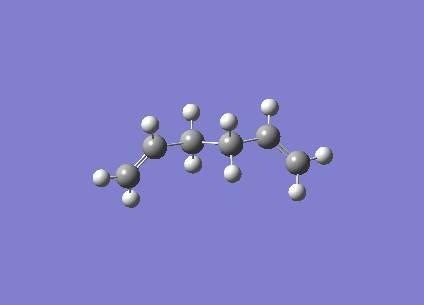
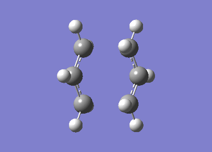
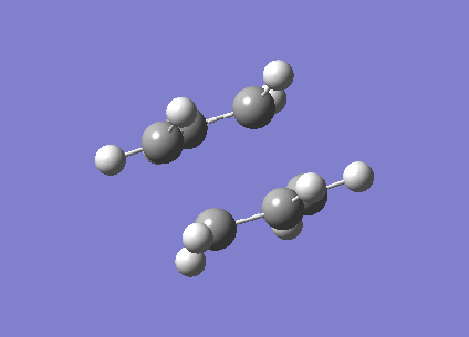
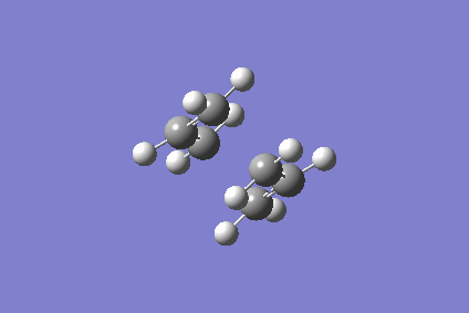
There are several different conformations of the 1,5 hexadiene because there is free rotation around the C-C single bonds. Each of these different conformation has a different energy due to the interactions of the chain and the effect of there entropy.
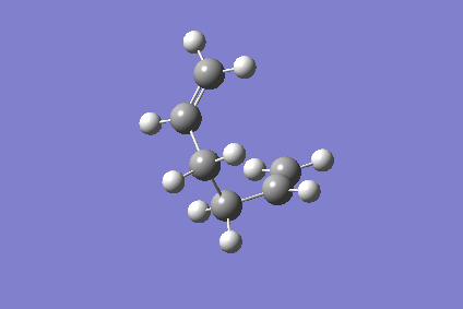
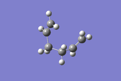
There are 10 different conformations of the 1,5 - hexadiene compounds due to the antiperiplanar(or gauche/synclinal) arrangements and synperiplanar( or Anticlinal) arrangements. The compounds were analysied using the HF and the 3-21 basis set. The results are shown in the table below with thier log files. The conformations are also ranked into an order related to their stability.
| Conformation | Structure | Point Group | Energy, Ha | Energy Relative to most stable, kcalmol-1 | Stability Rank |
|---|---|---|---|---|---|
| Anti 1[2] | C2 | -231.69260 | 0.038 | 2 | |
| Anti 2[3] | Ci | -231.69254 | 0.075 | 3 | |
| Anti 3[4] | C2h | -231.68907 | 2.253 | 9 | |
| Anti 4[5] | C1 | -231.69097 | 1.060 | 6 | |
| Gauche 1[6] | C2 | -231.68772 | 3.100 | 10 | |
| Gauche 2[7] | C1 | -231.69167 | 0.621 | 4 | |
| Gauche 3[8] | C1 | -231.69266 | 0.000 | 1 | |
| Gauche 4[9] | C2 | -231.69153 | 0.709 | 5 | |
| Gauche 5[10] | C1 | -231.68962 | 1.908 | 7 | |
| Gauche 6[11] | C1 | -231.68916 | 2.196 | 8 |
1 Ha = 627.5 kcal mol-1
The method used to calculate the energies of the conformations is basic as it does not consider the electron correlation.
There is not a noticeable trend in the data which suggest that the gauche or anti configuration are more stable. Of all the conformations the gauche 3 conformer was the most stable. This is unexpected as the anti arrangements of small molecules are normally more stable; for example for butane the anti conformer is significantly (2kcal mol-1[12]) more stable than the gauche conformer. This unexpected result may be due to the electron richness of the hexadiene species which affects the Van der Walls attractions between parts of the conformer.
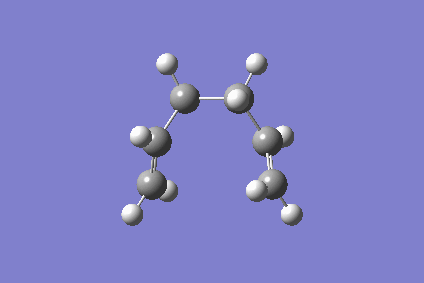
The three most stable conformations are analysed using the DFT/B3LYP method and using a 6-31G* basis set in order to optimise the structure more accurately. Each conformation is shown with its Newman projection in order to show the structure in another way. It is important to compare all three of the conformations using the same method and basis set.
Again the log files and energies of the comformors are shown below. The relative energies and energy 'rank' are shown.
| Conformation | Structure | Newman Projection | Point Group | Energy, Ha | Energy Relative to most stable, kcalmol-1 | Stability Rank |
|---|---|---|---|---|---|---|
| Gauche 1 [13] |  |
C1 | -234.61133 | 0.282 | 3 | |
| Anti 1 [14] |  |
C2 | -234.61171 | 0.000 | 1 | |
| Anti 2 [15] |  |
Ci | -234.61171 | 0.044 | 2 |
There is no large change in the structures of the reoptimised conformers for this method and basis set. The results of this calculation agree more strongly with the expected results which would show that the anti arrangements are lower in energy. The lowest energy conformer is anti 1, which is due to the stabilising effect caused from the overlapping of the antiperriplanar allyl sigma orbitals. In addition there is less strain between the two allyl groups at either end of the molecule in the anti conformations. The repulsion is due to the Pauli repulsion which occurs when atoms get too close together.
Although there were no large changes in the structure of the molecule the dihedral angles of the terminal carbons has changed slightly. For example when analysed using the HF method the angles are 124.8o and when analysied with the DFT method they are 125.3o.
Therefor as a result of the these two optimisation methods it can be seen that the HF has a much smaller level of accuracy compared tot he DFT. However the HF method can still be used to form a rough guide to the stabilities of each conformation.
Infrared Analysis of 1,5 Hexadiene Conformations
To see if the optimisation has been completed fully the low energy vibrations of the molecule are investigated. It is possible to see if the optimisation has been completed to a minima by seeing the frequency of the low vibrations. If the vibrations are negative (normally less than -10 cm-1 is considered negative due to errors from the calculations) then the optimisation has not been completed as the energies have not fully converged.
From analysis of the frequency data it can be seen that all the conformations have no negative vibrational modes and therefore have converged to the geometric energy minima. The three infrared spectrums are shown below and the vibrational log files are provided, anti 1[16], anti 2[17] and gauche 3[18].
| Anti 1 | Anti 2 | Gauche 3 |
 |
 |
 |
The vibrational analysis of the molecule shows that there is a difference from the literature[19]. The C-H bond and C-C bond stretches occur in the expected region but there is part of the infrared spectrum which shows stretches about 1730cm-1. These peaks are attributed to the C=C stretches, but these peaks are normally observed at in the mid 1600s cm-1.
The two different stretches are shown in the table below. The symmetrical C=C stretch involes the two C=C stretches occuring at the same time as each other whereas the asymmetric C=C stretch involves the two different C=C stretches occurring at different times. The animations of the stretches can be seen using the anti 1 conformation as an example.
| Conformer | Symmetrical Stretch cm-1 [Intensity] | Assymmetrical Stretch cm-1 [Intensity] |
|---|---|---|
| Anti 1 | 1732 [4.73] Show Vibration | 1735 [13.6] Show Vibration |
| Anti 2 | 1731 [0] Show Vibration | 1734 [18.1] Show Vibration |
| Gauche 3 | 1732 [6.89] Show Vibration | 1733 [6.13] Show Vibration |
Thermochemical Analysis of 1,5 Hexadiene Conformations
The thermochemical data for each conformation can be obtained as a result of the vibrational analysis using the DFT/B3LYP method with the 6-31G* basis set. The log files of the calulations are shown above.
The data below shows the values for the anti 1 conformation. The values in the table show the different energy parameters which are being considered.
This shows the energy of the anti 1 conformation at 298.15K and 1 atm.
 Zero-point correction=                           0.142466 (Hartree/Particle)
 Thermal correction to Energy=                    0.149804
 Thermal correction to Enthalpy=                  0.150749
 Thermal correction to Gibbs Free Energy=         0.111533
 Sum of electronic and zero-point Energies=           -234.469318
 Sum of electronic and thermal Energies=              -234.461979
 Sum of electronic and thermal Enthalpies=            -234.461035
 Sum of electronic and thermal Free Energies=         -234.500250
This shows the energy of the anti 1 conformation at 0K (0.0001K).
 Zero-point correction=                           0.142903 (Hartree/Particle)
 Thermal correction to Energy=                    0.142903
 Thermal correction to Enthalpy=                  0.142903
 Thermal correction to Gibbs Free Energy=         0.142903
 Sum of electronic and zero-point Energies=           -234.468881
 Sum of electronic and thermal Energies=              -234.468881
 Sum of electronic and thermal Enthalpies=            -234.468881
 Sum of electronic and thermal Free Energies=         -234.468881
By comparing the values from the log file the amount of energy from the thermal excitations can be seen. The anti 1 at 0K shows no difference in the energy when thermal energy was taken into account compared to when it was not. This is because it is run at 0K and therefore has no thermal energy and therefore this is the zero point energy.
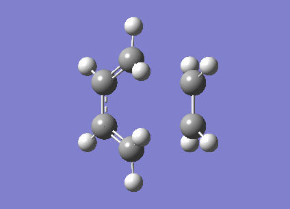
Optimising the Chair and Boat Transition States
The transition state of the Cope rearrangement can occur via the chair or the boat conformations. Both of these transition states contain the CH2CHCH2 fragments.
Chair conformation
The chair conforamtion transition state is optimised in two different ways.
Method 1 uses a Hessian matrix that is changed at each optimisation step.
Firstly the two allyl fragments are orientated into a chair orientation and then optimised to a TS(Berny). This optimisation uses the Hartree-Fock method and the 3-21g basis set.
The log file of the calculation is provided[20]. When the molecule is vibrationally analysed there is an imaginary vbration at -817.96cm-1 (show vibration). This vibrational mode was expected and confirms the molecule has been optimised correctly.
The distance between the terminal carbons was set to approximatly 2.2Â however this distance has reduced to 2.02Â and 202Â respectively.
The graph below shows how the total energy of the structure changes as the molecules geometry is moved(top) and how the route mean square of the gradient as the molecules geometry changes.

Method 2 requires the freezing of the reaction coordinate and the rest of the molecule is optimised around these constraints.
The log file of the calculation is provided[21]. Again, when the molecule is vibrationally analysed there is an imaginary vbration at -818.03 cm-1 (Show Vibration). This vibrational mode was expected and confirms the molecule has been optimised correctly.
The distances between the terminal ends of the allyl fragments are 2.02Â and 2.02Â respectively. This has decreased from the 2.2Â which was originally specified. These are the same values (when rounded to 3sf) as are made from method 1. This in addition to the vibrational analysis shows that the transition state has been modeled in both cases.
Boat Conformation
The conformation transition state can be calculated in several different ways. The first uses the QTS2 method where the atoms are labeled and placed in a specific order.
The calculation was carried out on the reactant and product when they were both in the anti1 geometry. This is not the correct geometry of the transition center and therefore the calculation did not work [22].
The geometry of the reactants and products is them changed so that the cetral 4 carbon atoms have a dihedral angle of 0o and each sp3 hybridised carbon and the carbons on either side have a bond angle of 100o. The calculation is run again and it was successful, the log file is provided[23].
The structure is optimised using the QST2 method and the structure is shown below. The distance between the terminal carbons is 2.14Â which is large than the distance observed in chair conformation.
Intrinsic Reaction Coordinate Analysis of the Chair and Boat Transition States
The intrinsic reaction coordinate tracks a reaction as it moves from the high energy transition state to a lower energy more stable product. As the arrangement and geometry of the molecule is changed it follows the lowest energy and forms a potential energy surface.
There are 4 different methods which can be used in order to calculate the intrinsic reaction coordinate of a molecule.
Method 1 This first method is the standard used and is not specific to a molecule. As a result this method may need to be altered in order to gain a full understanding of the minimum energy pathway.
50 points along the pathway are computed and related to the collapse of the chair transition state for the forward reaction only. The log files for the calculations are provided chair[24] and boat[25]. For the chair conformation the calculation was not able to complete and as a result the stepsize was changed to five, by adding irc=stepsize=5 to the key words.
The table below shows the summary of the IRC optimiastion.
| Conformer | Total Energy, Ha | RMS Gradient |
|---|---|---|
| Chair | -231.61932 | 0.00003114 |
| Boat | -231.51103 | 0.0041641 |
The graphs below shows the how the total energy of the molecule changes after each step and the RMS gradient for the chair conformation.
Method 2
This method optimises the final step of the IRC calculated in method 1. The Hartree-Fock method and the 3-21G basis set are used. The log file for the optimisations are provided, chair[26] and boat[27].
The energy of the chair conformation is -231.69167 and the energy of the boat conformation is -231.68916.
Method 3
This method is a variation on method. Instead of 50 steps being recorded, 100 steps are recorded. This means there are more points of the graph shown in method because the starting and end points on the graph will remain the same. The log files of the calculations are provided, chair and boat[28].
| Conformer | Total Energy, Ha | RMS Gradient |
|---|---|---|
| Chair | -231.61932 | 0.00003114 |
| Boat | -231.68740 | 0.0002376 |
Method 4
This method calculates the force constant at each step instead of at the start. Again the start and end points of the graph are the same. The log files are supplied, chair[29] and boat[30].
| Conformer | Total Energy, Ha | RMS Gradient |
|---|---|---|
| Chair | -231.68868 | 0.0006730 |
| Boat | -231.65475 | 0.006217 |
Summary
| Conformer, Method and Log File | Maximum Number of Steps | Compute Force Constant | Terminated After Step | Total Energy | RMS Gradient |
|---|---|---|---|---|---|
| Chair, 1 | 50 | Once | 51 | -231.69167 | -0.0000314 |
| Chair, 2 | N/A(opt) | Once | N/A(opt) | -231.69167 | 0.00000268 |
| Chair, 3 | 100 | Once | 70 | -231.61932 | 0.0006217 |
| Chair, 4 | 50 | Always | 70 | -231.68868 | 0.0.0000314 |
| Boat 1 | 50 | Once | 51 | -231.51103 | 0.004164 |
| Boat 2 | N/A(opt) | Once | N/A(opt) | -231.68916 | 0.00000283 |
| Boat 3 | 100 | Once | 101 | -231.68740 | 0.0002376 |
| Boat 4 | 50 | Always | 51 | -231.65475 | 0.006217 |
Activation Energies
The activation enengies for the chair and the boat conformers can be calculated for the structure calculated using HF/3-21G, which is a less accurate method and DFT-B3LYP/6-31* which is more accurate. If any differences are present they can be compared in order to analysis the different methods.
The activation energy is the highest energy structure on the reaction path. For each method the lowest energy conformer was used, so the gauche 3 conformer was used for the HF/3-21G minimisation and for the DFT-B3LYP/6-31* metod the anti 1 conformer was used. The values obtained we convereted in to kcal mol-1 by multiplying by 627.5.
| Conformer | HF/3-21G Method - Electronic and Zero point energy | HF/3-21G Method - Electronic and Thermal energy | Activation energy at 298.15K, kcal mole-1 | Activation energy at 0.0001K, kcal mole-1 | DFT-B3LYP/6-31* Method - Electronic And Zero Point Energy | DFT-B3LYP/6-31* Method - Electronic And Thermal Energy | Activation energy at 298.15K, kcal mole-1 | Activation energy at 0.0001K, kcal mole-1 | Literature activation energy, kcal mol-1 |
|---|---|---|---|---|---|---|---|---|---|
| Chair | -231.46670 | -234.46888 | 45.98 | 48.64 | -234.46932 | -234.46888 | 37.57 | 38.46 | 33.5 ± 0.5[31] |
| Boat | -231.44153 | -231.44172 | 52.31 | 55.74 | -234.40121 | -234.39341 | 46.45 | 45.98 | 44.7 ± 2.0[32] |
The energies calculated for the transition states do not match the literature energies because they are too large. However the difference between the two structures is similar to the literature values.
As can be seen from the energies of the transition states the more advanced method(DFT-B3LYP/6.31*) produced results which are closer to the literature activation method. Therefor this method should be used in order to calculate the energies of transition states.
Diels Alder Cycloaddition
Introduction

A Diels Alder reaction is a cycoladdition reaction similar to the dimerisation of cyclopentadiene investigated in module 1. This reaction involves the reaction of butadiene and ethene to form cyclohexane. These forms of reaction are very usful in synthetic chemistry as they are a neat way of forming 6 memebered rings.
The Diels Alder reaction is a π4s + π2s cycloaddition, where the π orbitals of the diene are electron poor and the π orbitals of the ene are electron rich.
In this part of the module two different Diels Alder reactions are investigated. Firstly the reaction between cis-Butadiene and ethene and secondly between cyclohexadiene and maleic anhydride.
Optimiseing the Reactants
The reactants are drawn unsing gaussview and then optimised using the AM1 semi-emprical method. This method is the middle ground between HF/(less accurate) and DFT-B3LYP(more accurate) methods.
The total energy and the RMS gradient are presented in the table below and the log files are provided, cis-butadiene[33] and C[34].
| Compound | Energy | RMS Gradient | Structure |
|---|---|---|---|
| Cis-Butadiene | 0.04880 | 0.0001248 | |
| Ethene | 0.02619 | 0.00003328 |
After the structures of the compound have been minimised the molecular orbitals of the HOMO and LUMO of each complex are visualized. These orbitals are important as they are the frontier orbitals and involved in the reaction.
| Compound | HOMO | LUMO | MO Diagram |
|---|---|---|---|
| Cis-Butadiene |  |
 |
 |
| Ethene |  |
 |
 |
By looking at the HOMO and LUMO of the two molecules the symmetry between them can be seen. It is interesting to compare the LUMO of the cis-butadiene and the HOMO of ethene (or the other two orbitals) because the orbitals overlap in phase with each other and therefore are possible reaction paths.
Optimising the Transition State
The Optimised transition state of the reaction will have the largest orbital overlap between the two molecules. The cyclic tranistion state is constructed using the frozen coordinate method which used because it is reliable.
The distance between the two terminal carbons is set to 2.20Â and the geometry is optimised using the AM1 method. The bond between the terminal carbons in then unfrozenand the AM1 optimisation was carried out again. In addition to the AM1 method the DFT-B3BYP/6-31G* is also carried out to allow a comparison to be made.
The table below shows the infrared spectrums of the transition states optimised using both methods.
| AM1 Optimised | DFT-B3LYP/6-31G* Optimised |
|---|---|
 |
 |
The AM1 optimised spectrum shows an imaginary vibration at -818.19 cm-1(show vibration). This shows that the molecule has been successfully optimised to the transition state. An imaginary vibration was also seen in the DFT optimised structure at -525.86 cm-1(show vibration) which again shows that this method successfully optimised the transition state.
The energies, frequencies and log files of the calculations are shown in the table below.
| Transition State and Log File | Total Energy, Ha | RMS Gradient | Imaginary frequency vibration, cm-1 [Intensity] |
|---|---|---|---|
| AM1 Optimised[35] | -231.60320 | 0.00003731 | -818.19 [9.3561] |
| DFT B3LYP/6-31G* | -234.54390 | 0.00006444 | -525.86 [5.8373] |
The bond lengths of the transition states when optimised using the two methods are measured and presented below.
| Optimisation Method | Distance Between Terminal Carbons, Â | Butadiene C=C Bond Length, Â | Butadiene C-C Bond Length, Â | Ethene C=C, Â |
|---|---|---|---|---|
| AM1 Optimised | 2.2094 | 1.3640 | 1.3945 | 1.3758 |
| DFT/B3LYP Optimised | 2.2702 | 1.3833 | 1.4069 | 1.3861 |
When the bond lengths on the diene are compared to each other it is found that the C=C and C-C bond contained in the diene are approximatly the same length. This is true for both of the methods. The bond lengths are the same because the butadiene molecule is a conjugated π systemand as a result the bond lengths will be similar. Therefore this implies that the transition state is also a conjugated π system.
The only major difference between the structures of the molecule arises from the distance between the terminal carbons, where the bond is formed between. The difference arises from the assumptions used in each calculation. The semi empirical method may not account for the repulsion between the two atoms and therefore show a smaller inter-nuclei distance.
The HOMO and LUMO of the transition states are analysised for both methods and the visualisations of the orbitals can be seen.
| Optimisation Method | HOMO | LUMO | Molecular Orbital Diagram |
|---|---|---|---|
| AM1 Optimisation |  |
 |
 |
| DFT-B3LYP/6-31G* Optimisation |  |
 |
 |
The molecular orbitals of the HOMO and the LUMO are different as a result of each optimisation. This is because the two methods use different assumptions and the effect of them can be seen in the structure of the molecular orbitals. The different structures cause the energy of the molecular orbitals to change. The different assumptions which are taken into account for each method cause different orbitals to mix which causes the different HOMO and LUMO structures and energies.
Optimising the Reactants of Cyclohexadiene and Maleic Anhydride
Another simple Diels Alder reaction involves maleic anhydride and cyclohexadiene and can form two different isomer products. The endo and exo products form under different reaction conditions. The endo reaction forms under kinetic control at low temperatures and short reaction times and the exo forms when the reaction time is longer and the temperature is high.

The reactants of the Diels Alder reaction were optimised using the semi emperical method, AM1. The energies of the compounds and the RMS gradients are shown below in the table. The log files for the Cyclohexadiene[36] and Maleic Anhydride[37] are provided.
| Compound | Energy | RMS Gradient | Structure |
|---|---|---|---|
| Cyclohexadiene | 0.1028 | 0.0000 | |
| Maleic Anhydride | -0.1218 | 0.0000112 |
The structures of two reactants were simple to optimise and produced an accurate structure.
The HOMO and LUMOs of the reactants are shown in the table below along with the MO diagram.
| Compound | HOMO | LUMO | MO Diagram |
|---|---|---|---|
| Cyclohexadiene |  |
 |
 |
| Maleic Anhydride |  |
 |
 |
Optimising the Transition States of Cyclohexadiene and Maleic Anhydride
The transition states of both the endo and exo complex were formed using the frozen coordinate method. The DFT-B3LYP method was used in order to calculate the energies of the transition states. This method was used because it is more accurate than the AM1 method originally used in the previous Diels Alder calculation. The results of the calculations are shown in the table below.
The transition states of both the endo and exo calculations are shown in the table below. The log file of each transitions state is provided.
| Transition state | Total Energy | RMS Gradient | Structure |
|---|---|---|---|
| Endo | -612.683 | 0.00000558 | |
| Exo | -605.604 | 0.00000325 |
The results for the endo and exo are shown above. It can be seen that the endo transition state is more stable than the exo, whch is expected because the endo product is the thermodynamic product of the reaction.
The frequency analysis of both the transition states shows there is an imaginary vibration in the region characteristic to a transition state.
| Transition State | Imaginary vibration cm-1 | Infrared spectrum |
|---|---|---|
| Endo | -542.23 |  |
| Exo | -647.46 |  |
The presence of the imaginary vibrations in the structure shows that a transition state has been formed.
| Transition State | New bond C-C length, Â | Cyclohexadine C=C bond length, Â | Cyclohexadine C-C bond length, Â | Maleic Anhydride C=C bond length, Â | Maleic Anhydride C=O bond length, Â |
|---|---|---|---|---|---|
| Endo | 2.2684 | 1.3913 | 1.4031 | 1.3940 | 1.2017 |
| Exo | 2.2606 | 1.3700 | 1.3976 | 1.3731 | 1.1912 |
The bond lengths from the optimised tranistions state dont show a large difference between the two transition states. The difference in the approach angles does not change how the reaction behaves.
The molecular orbitals of the HOMO-1, HOMO, LUMO and LUMO+1 are shown below. These orbitals were chosen in order to understand the transition state.
| Transition State | HOMO -1 | HOMO | LUMO | LUMO +1 |
|---|---|---|---|---|
| Endo |  |
 |
 |
 |
| Exo |  |
 |
 |
 |
The LUMO +1 orbital shows that there is secondary orbital overlap between the orbitals from the carbonyl carbons. The endo orbitals are in the correct orientation to interact and therefore lower the energy of the transition state.
References
- ↑ Arthur C. Cope; et al.; J. Am. Chem. Soc. 1940, 62, 441.
- ↑ http://hdl.handle.net/10042/to-13312
- ↑ http://hdl.handle.net/10042/to-13313
- ↑ http://hdl.handle.net/10042/to-13314
- ↑ http://hdl.handle.net/10042/to-13315
- ↑ http://hdl.handle.net/10042/to-13336
- ↑ http://hdl.handle.net/10042/to-13337
- ↑ http://hdl.handle.net/10042/to-13340
- ↑ http://hdl.handle.net/10042/to-13341
- ↑ http://hdl.handle.net/10042/to-13342
- ↑ http://hdl.handle.net/10042/to-13343
- ↑ H. Rzepa, 2nd Year Conformational Analysis Course, 2011, p. 'Alkanes', http://www.ch.ic.ac.uk/local/organic/conf/
- ↑ http://hdl.handle.net/10042/to-13378
- ↑ http://hdl.handle.net/10042/to-13379
- ↑ http://hdl.handle.net/10042/to-13380
- ↑ http://hdl.handle.net/10042/to-13381
- ↑ http://hdl.handle.net/10042/to-13382
- ↑ http://hdl.handle.net/10042/to-13383
- ↑ J. Coates, Encyclopaedia of Analytical Chemistry, R. A. Meyers (Ed.), 2000, pp. 10815-10831
- ↑ http://hdl.handle.net/10042/to-13399
- ↑ http://hdl.handle.net/10042/to-13426
- ↑ http://hdl.handle.net/10042/to-13465
- ↑ http://hdl.handle.net/10042/to-13466
- ↑ http://hdl.handle.net/10042/to-13443
- ↑ http://hdl.handle.net/10042/to-13433
- ↑ http://hdl.handle.net/10042/to-13715
- ↑ http://hdl.handle.net/10042/to-13716
- ↑ http://hdl.handle.net/10042/to-13738
- ↑ http://hdl.handle.net/10042/to-13743
- ↑ http://hdl.handle.net/10042/to-13742
- ↑ 3rd Year Computational Chemistry Online Lab Manual, Module 3, 2011
- ↑ 3rd Year Computational Chemistry Online Lab Manual, Module 3, 2011
- ↑ http://hdl.handle.net/10042/to-13516
- ↑ http://hdl.handle.net/10042/to-13514
- ↑ http://hdl.handle.net/10042/to-13668
- ↑ http://hdl.handle.net/10042/to-13722
- ↑ http://hdl.handle.net/10042/to-13720