Rep:Mod3:p.thakrar

Module 3 - Physical Computational Techniques

The Cope Rearrangement

The Cope rearrangement is a [3,3]-sigmatropic reaction involving the concerted migration of a group from one point of attachment to another. In the process one σ bond is broken and another is made within a conjugated π system. The Cope rearrangement to be investigated is that of 1,5-hexadiene as illustrated in Figure 1.

Fig. 1 - Cope Rearrangement Mechanism

Optimizing the Reactants and Products

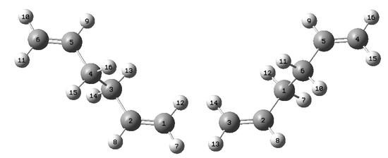
In Gaussview, a molecule of 1,5-hexadiene was drawn in the antiperiperiplanar conformation, with a dihedral angle between the four central carbon atoms of approximately 180^o. A second 1,5-hexadiene molecule was drawn in a gauche conformation with a dihedral angle of 60^o. These structures were then 'cleaned' before being optimised using the Hartree-Fock method and a basis set of 3-21G. These optimizations resulted in the ‘anti 3’ and ‘gauche 3’ geometries respectively as illustrated in Table 1 and Table 2 below which also include some of the key information obtained from the summary of each molecule. Various alterations were made to the structure of the molecule whilst still keeping them in the correct antiperiplanar or gauche conformations. These structures were identified using Appendix 1 and can also be seen in the tables below.

Table 1 - Antiperiplanar

Calculation Type	FOPT	FOPT	FOPT
Calculation Method	RHF	RHF	RHF
Basis Set	3-21G	3-21G	3-21G
Final Energy/a.u.	-231.69260	-231.69254	-231.68907
RMS Gradient Norm/a.u.	0.00001559	0.00003092	0.00001163
Dipole Moment/Debye	0.2023	0.0008	0.0001
Point Group	C2	Ci	C2h

Table 2 - Gauche

Calculation Type	FOPT	FOPT	FOPT
Calculation Method	RHF	RHF	RHF
Basis Set	3-21G	3-21G	3-21G
Final Energy/a.u.	-231.68772	-231.69266	-231.69153
RMS Gradient Norm/a.u.	0.00000556	0.00002098	0.00001063
Dipole Moment/Debye	0.4557	0.3407	0.1218
Point Group	C2	C1	C2

It would be assumed that the gauche conformers would, in general, have a higher energy due to the increased steric clash. However, comparison of the most stable anti conformer with the most stable gauche, shows the opposite with the gauche being more stable by 0.32 kJ mol^-1 (0.00012 Hartree). This indicates that another factor determines the energy of the conformers and is larger than the opposing energy resulting from the steric repulsion. Consideration of the bonding interactions within the dialkene may help explain the reversal in expected energies. A favourable donation from the C=C π orbital into the C-H σ* orbital results in a stabilisation of the Gauche 3 conformer which explains the observed data.

The 'Anti 2' conformation was then further optimized using the density functional theory B3LYP method and 6-31G(d) method. This runs a more accurate simulation and yields a better approximation of the geometry and optimization of the molecule. The data obtained for the initial optimization using the Hartree-Fock method is presented in Table 3 below along with the results using DFT. However, these results cannot be compared due to the different methods used in each of the calculations.

Table 3: Anti2 - HF vs DFT

Method	Structure	Energy/a.u.
HF/3-21G		-231.69254
DFT/B3LYP/6-31G(d)		-234.61171

Table 4: Anti2 - HF vs DFT

	Dihedral Angle/o			Bond Length/Å
	HF/3-21G	DFT/B3LYP/6-31G(d)		HF/3-21G	DFT/B3LYP/6-31G(d)	Literature
14-12-1-8	-114.65328	-118.58102	14-12	1.316	1.334	1.340
12-1-8-6	-179.99319	-179.95143	12-1	1.509	1.504	1.508
-	-	-	1-8	1.553	1.548	1.538

Table 3 and 4 show that using the higher accuracy basis set and method results in a change in geometry. Comparison of the bond lengths shown in Table 4 with the literature values shows the higher accuracy DFT method to have more accurate results compared to those obtained via the lower accuracy Hartree-Fock method. The dihedral angle for C14-C12-C1-C8 is also larger (and assumed more accurate) for the DFT method. One final observation gleaned from Table 3 is the energy. The DFT method has yielded a lower energy isomer indicating that the method provides a more accurate optimized geometry.

Frequency Analysis of Reactants and Products

A frequency analysis is useful in determining whether a minimum in the optimized geometry has been calculated. This can be found by looking at the frequencies for the system; if all are positive a minimum has been obtained, if one is negative then the system is at a transition state and if more than one is negative, the calculation has failed to find a critical point and the optimization has failed. A frequency analysis was carried out on both the Hartree-Fock and DFT optimized structures.

The frequency analysis for the Hartree-Fock optimized geometry produced negative frequencies showing that a minimum had not been reached. However, as expected, the higher accuracy optimization method did yield a minimum with all positive frequency values.

The frequency analysis can also be used to obtain thermodynamic information contained within the log file. The calculation was carried out at 298.15 K and was re-run to find the data at absolute 0 temperature.This was obtained by re-running the frequency calculation for the Anti2 DFT optimised structure with the additional keywords: ‘Freq=ReadIsotopes’. The input file was also manually edited before the calculation was run. Initially, the temperature was set to 0.001 K as Gaussview would read 0.0 to be a default and would therefore take the temperature as the standard 298.15 K. However, on inspection of the output file, the energies were different which was not expected. On further inspection it was found that Gaussview had carried out the calculation at 12 K which could have resulted from Gaussview reading the mass of carbon instead of the temperature. Hence the calculation was repeated but this time using 0.000001 for the temperature but when the calculation was run, Gaussian kept reporting an error. No errors could be found within the input file so the calculation was repeated, this time using Gaussian and the checkpoint file. The temperature was once again set to 0.001 K and Gaussian returned corrections corresponding to the four different energies in the table. All the calculated energies can be seen in Table 5 below:

Table 5

	298.15 K/a.u.	12 K/a.u.	0 K/a.u.
Sum of Electronic and Zero-point Energies	-234.469183	-234.429607	-234.48444
Sum of Electronic and Thermal Energies	-234.461844	-234.426493	-234.48444
Sum of Electronic and Thermal Enthalpies	-234.460900	-234.429455	-234.48444
Sum of Electronic and Thermal Free Energies	-234.500735	-234.430232	-234.48444

The energies detailed in Table 5 are representative of different parameters:

• Sum of Electronic and Zero-point Energies – is the potential energy at 0 K including the zero-point vibrational energy: E = E_elec + ZPE
• Sum of Electronic and Thermal Energies – is the energy at 298.15 K and 1 atm. Includes contributions from the translational, rotational and vibrational energy modes occurring at this temperature: E = E + E_vib + E_rot + E_trans
• Sum of Electronic and Thermal Enthalpies – this contains an additional correction for RT which is important when analysing dissociation reactions: H = E + RT
• Sum of Electronic and Thermal Free Energies – this includes the entropic contribution to the free energy: G = H - TS

The data shows that as the temperature decreases, the stability of the conformer also decreases as each of the energies becomes more positive. It is also important to note that all the energies at absolute 0 are the same as any thermal contributions will be zero and therefore each of the energies will be comprised solely of the electronic and zero point energies. At 298.15 K and also 12 K, the sum of electronic and thermal free energies is more stable in comparison to the other three energies. This can be attributed to the temperature dependant entropy term which has now been taken into account.

Optimizing the "Chair" and "Boat" Transition Structures

The next step of the investigation looks into the structures of the transition states of which there are two; a chair conformer with C_2h symmetry and a boat conformer with C_2v symmetry. These structures can be found in Appendix 2.

Initially a CH₂CHCH₂ fragment was drawn in Gaussview and optimized using the HF/3-21G level of theory. This optimized fragment was then used to create a rough chair transition state as shown in Appendix 2 with an approximate bond distance between the terminal carbon atoms of 2.2 Å. This structure was optimized by selecting Opt+Freq in the calculation window and then selecting ‘Optimization to a TS (Berny)’. The force constant was altered to calculate once and ‘Opt=NoEigen’ was inserted into the additional keywords box. This stops the calculation aborting if more than one imaginary frequency is found during the optimization which can happen if the guessed structure is inaccurate.

This structure was further optimized using the frozen coordinate method. Under the Edit menu, Redundant Coord Editor was selected and two of the terminal carbon atoms on the allyl fragment were highlighted. The settings of the Redundant Coord Editor was changed from Unidentified and Add to Bond and Freeze Coordinate respectively. This process was repeated for the second set of terminal carbon atoms and the optimization was run.

Table 6

	Optimised Through a TS (Berny)	Optimised Through a Frozen Coordinate Method
Optimised TS Structure
Terminal C-C bond length/Å	2.02	2.02
Energy/a.u.	-231.6193	-231.6193
Imaginary Frequency/cm-1	-818	-818
Animation	Vibration	Vibration

The data in Table 6 shows that both methods result in the same chair transition state structure. The energy difference between the two structures was identical to 4 decimal places and a difference was only observed at 6 decimal places giving a negligible difference between the two. Another property indicating both structures are identical was the bond distances between the terminal carbon atoms which were found to be 2.02 Å. The imaginary vibrations shown were found to be -818 cm^-1 in both structures and show that the making and breaking of bonds occurs in a concerted manner. This is expected for a pericyclic reaction where one bond forms as another bond breaks.

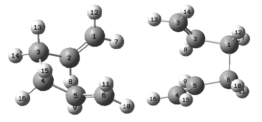
The boat transition state structure was also optimized, but this time using the QST2 method. This method allows the reactants and products for a reaction to be specified and the calculation interpolates between the structures to try and find a transition state. The atoms in the reactants and products have to be numbered in the same way, which requires manual alteration of the product so that it corresponds to the numbering on the reactant. The optimized anti2 structure was opened in Gaussview and the structure was copied in order to read multiple geometries; which allowed structures to be viewed simultaneously making it easy to see which numbers needed to be edited in the product structure. This was carried out by selecting Labels under the View menu followed by Atom List under the Edit menu. It was then possible to click on each of the individual atoms and renumber them. Both structures can be seen in Figure 2 below.

Fig. 2

An optimization and frequency QST2 calculation was then run on the structures. However, it was found that the calculation failed and produced a structure similar to a chair transition state but more dissociated. This resulted from translation of the top allyl fragment during the linear interpolation calculation. Gaussian did not consider the possibility of rotation around the central bonds. As a result, the structures were altered to that shown in Figure 3, where the central dihedral angle (C2-C3-C4-C5) is 0^o and the inside angles (C2-C3-C4 and C3-C4-C5) were reduced to 100^o.

Fig. 3

These structures were then used to repeat the calculation, the results of which can be seen in Table 7 below:

Table 7

	Optimised Using QST2
Optimised TS Structure
Terminal C-C bond length/Å	2.14
Energy/a.u.	-231.60280
Imaginary Frequency/cm-1	-840
Animation	Vibration

The imaginary frequency present at -840 cm^-1 shows that a transition state has been found. For the boat transition structure, the frequency is more negative compared to that of the chair but still shows simultaneous bond making and breaking between the terminal carbon atoms. Comparison of the animations shows the vibration to be acting in the same manner. The distance between the terminal carbons however, is longer in this structure relative to the chair. This is reflected in the energies as the chair transition state has a slightly lower energy than that found for the boat structure.

The method used to optimize the boat transition structure is more tedious than the TS(Berny) method used for the chair conformer as renumbering the atoms in the correct manner takes a substantial amount of time. If the atoms were numbered wrong, the optimization would fail which required the atoms to be further renumbered. This was not required for the Berny method hence making it more time efficient.

Intrinsic Reaction Coordinate Method

It is almost impossible to predict which product the chair or boat transition state will lead to. The Intrinsic Reaction Coordinate (IRC) method can be used in Gaussian to solve this problem. IRC allows the minimum energy path from a transition structure down to its minimum on a potential energy surface to be followed. This process creates a series of points by taking small geometry steps in the direction where the slope of the potential energy surface is steepest.

The first step was to open the chair transition structure in Gaussview. A Gaussian calculation was run and IRC was selected under the Job Type. The reaction coordinate was set to compute in the forward direction due to the symmetrical properties of the molecule. The number of points along the IRC was changed to 50 and the force constant was set to once. The results of this calculation can be seen in Table 8 below.

The calculation in which the force constants are assumed constant and therefore only calculated once does not seem to have reached a minimum on the potential energy surface. This can be confirmed by looking at the RMS gradient along the IRC which would have been expected to finish close to 0. A final confirmation that the minimum has not been reached is proven by the energy of the final structure. This energy does not correspond to any of the conformers calculated earlier or those given in Appendix 1 indicating that none of the given structures have been found.

In order to obtain a minimum geometry, one of three further methods could be carried out on the IRC product, each with its own advantages and disadvantages. The first of these is a minimization on the last point of the IRC, the second involves redoing the IRC calculation and specifying a larger number of points until a minimum is reached and the final involves restarting the IRC and specifying that the force constants will be calculated at each step. The first method is the fastest but can result in a wrong minimum if the geometry is not close enough to a local minimum. The second approach is more reliable but if too many points are specified than the wrong structure may be obtained by veering off in the wrong direction. The final method is the most reliable of the three but also the most expensive.

For this investigation the third method was used in order to find the minimum geometry was the final suggestion. This is because this is the most reliable method and although it is expensive, the system is relatively small. The results for this can also be seen in Table 8 along with the initial minimization.

Table 8

	Calculate Force Constants Once	Calculate Force Constants Always
Number of Points Along IRC	50	50
Final Structure
Energy/a.u.	-231.68043	-231.69134
IRC Pathway
IRC Gradient

The procedure was then repeated using the optimized boat transition state structure and the results can be seen in Table 9.

Table 9

	Calculate Force Constants Once	Calculate Force Constants Always
Number of Points Along IRC	26	50
Final Structure
Energy/a.u.	-231.67725	-231.68763
IRC Pathway
IRC Gradient

The number of points along the IRC was found to be 26 for the method where the force constant was only calculated once indicating that the molecule had fully converged before the full 50 points had been reached. However, comparison of the energy of the conformer with the energies provided in Appendix 1 showed this to be incorrect as the energy did not correspond to any of the conformers mentioned. As such the calculation was repeated using the calculate force constants always method which seemed to yield better results. It can be seen that the conformer is clearly gauche so comparison with Appendix 1 showed that gauche1 had been formed, with a difference of 0.00009 Hartree between the calculated value and the literature value.

Calculating Activation Energies

The final part of the Cope rearrangement investigation is calculation of the activation energies for the reaction via both transition structures. This involved reoptimizing the chair and boat transition structures using the B3LYP/6-31G (d) level of theory followed by frequency calculations to obtain thermodynamic information. Using the HF/3-21G optimized structures, an Opt+Freq calculation was carried out using the aforementioned level of theory. The results of this calculation can be seen in Table 10 below along with the thermodynamic information for the reactant and also the HF/3-21G optimized structures.

Table 10

	HF/3-21G			B3LYP/6-31G (d)
	Electronic Energy /a.u.	Sum of Electronic and Zero-point Energies (0 K) /a.u.	Sum of Electronic and Thermal Energies (298.15 K) /a.u.	Electronic Energy /a.u.	Sum of Electronic and Zero-point Energies (0 K) /a.u.	Sum of Electronic and Thermal Energies (298.15 K) /a.u.
Chair TS	-231.61932	-231.46671	-231.46134	-234.55699	-234.41492	-234.40901
Boat TS	-231.60280	-231.45092	-231.44530	-234.54309	-234.40233	-234.39600
Reactant (Anti2)	-231.69254	-231.53954	-231.53257	-234.61171	-234.46920	-234.46186

Subtracting the energy of the chair or boat transition structure from that of the anti2 reactant gives the activation energy of the chair or boat conformers respectively in Hartrees. This energy can be converted to kcal mol^-1 by multiplying by 627.509 for easier comparison with experimental data. The results can be seen in Table 11 below.

Table 11

	HF/3-21G (0 K)	HF/3-21G (298.15 K)	B3LYP/6-31G (d) (0 K)	B3LYP/6-31G (d) (298.15 K)	Expt. (0 K)
ΔE (Chair)/a.u.	0.07283	0.07123	0.05428	0.05285	-
ΔE (Chair)/kcal mol-1	45.70	44.70	34.06	33.16	33.5 ± 0.5
ΔE (Boat)	0.08862	0.08727	0.06687	0.06586	-
ΔE (Boat)/kcal mol-1	55.61	54.76	41.96	41.33	44.7 ± 2.0

The B3LYP/6-31G (d) method is more accurate so it would be expected to yield energies closer to the experimentally obtained values and comparison of the data in Table 11 shows this to be true. The energy for the boat conformer is slightly further out than the experimental value, even when the fluctuations due to errors are taken into account but this is not significant and could be attributed to errors in the calculation. The energies obtained using the HF method are significantly different to the experimental values showing how the lower level of theory does not provide a good enough estimate for the energies and therefore the structures. It does however, show the chair conformer to be lower in energy compared to the boat. This shows the advantages of using a low level of theory to optimize the structure first followed by a further optimization at a higher level of theory. It can also be seen that the chair conformer has a lower activation energy compared to the boat transition state by approximately 7.9 kcal mol^-1. This implies that the kinetic route for this reaction would proceed via the chair transition state which could be attributed to steric repulsions found in the boat conformer.

Now that the activation energies for both structures have been computed and compared it will be interesting to see how the structures of both molecules change using both the low and high levels of theory.

Table 12

	HF/3-21G Chair	B3LYP/6-31G (d) Chair	HF/3-21G Boat	B3LYP/6-31G (d) Boat
Optimised Structure
Energy/a.u.	-231.61932	-234.55699	-231.60280	-234.54309
Terminal C-C Bond Length/Å	2.02	1.97	2.14	2.21
C-C Bond Length/Å	1.39	1.41	1.38	1.39
Fragment Angle/o	120	120	122	122
Dihedral Angle/o	54.96	54.04	0.00	0.10
Imaginary Frequency/cm-1	-818	-545	-840	-531

As expected, using a higher level of theory results in a stabilization of the molecule. All other parameters besides the imaginary frequency do not see a significant change on using a higher level of theory. The frequencies obtained are the second derivative of the potential energy surface. The transition state occurs at a maximum and hence gives a negative frequency. The imaginary frequency does not represent a parameter specifically but the difference can be explained by the second derivative changing on using a different method.

Diels Alder Cycloaddition

This part of the investigation will use the aforementioned techniques to help characterise the transition state structures of a Diels Alder reaction. The reaction is a cycloaddition between a conjugated diene and a dienophile and may often be referred to as a [4s + 2s] cycloaddition. The π orbitals of the dienophile are used to form new σ bonds with the π orbitals of the diene. The reaction can occur in either a concerted stereospecific fashion (allowed) or not (forbidden) which depends on the number of π electrons involved. The reaction will be allowed if the HOMO of one species can interact favourably with the LUMO on the other. The reaction taking place is illustrated below:

Fig. 4

Optimizing the Reactants: Butadiene and Ethylene

The reaction illustrated in Figure X is a standard example of a Diels Alder reaction occuring between and and is further investigated in the following section. Initially, each of the structures were optimized using the semi-empirical AM1 method found on Gaussview. The HOMO and LUMO for each were then plotted and the symmetry for each considered in order to help determine whether or not the reaction is allowed.

Table 13

	1,3-Butadiene		Ethylene
	HOMO	LUMO	HOMO	LUMO
Molecular Orbital
Energy/a.u.	-0.343	0.017	-0.387	0.052
Symmetry	Antisymmetric	Symmetric	Symmetric	Antisymmetric

Table 13 shows visualisations of the HOMO and LUMO orbitals for both 1,3-butadiene and ethylene along with the corresponding energies and the symmetry of the orbital. It can be seen that the HOMO of butadiene and the LUMO of ethylene are both antisymmetric whereas the LUMO of butadiene and HOMO of ethylene are both symmetric. This implies that any possible interactions must take place between these specific sets of orbitals to maintain the orbital symmetry.

Optimizing the Transition State

The next step of the investigation involved looking into the transition state structure. Molecular orbital analysis of the optimized geometry can be used to determine if the previous statement regarding the reaction between orbitals of the same symmetry is correct.

The transition state is known to have an envelope type structure which maximizes the overlap between the ethylene π orbitals and the π system of butadiene. Initially, the optimized structures for butadiene and ethylene were copied into a new window in Gaussview before being rearranged to an envelope type structure with the ethylene slightly above the plane of the butadiene. The transition state optimization was carried out in two steps to prevent the calculation failing. The first of these was the frozen coordinate method where the distance between the terminal carbon atoms was set to 2.1 Å. This method locks the terminal carbon distance to that stated and allows the rest of the molecule to relax. This was then followed by an Opt+Freq calculation to a TS (Berny) which moves the two reactants closer together along the reaction coordinate resulting in a structure closer to that of the transition state. Two different methods were also tested, a lower accuracy method (semi-empiracal AM1) and the more accurate DFT/B3LYP/6-31G (d) level of theory. The results of each optimization can be seen in Table 14 below:

Table 14

Method	Semi-empirical/AM1 - Frozen Coordinate Method	Semi-empirical/AM1 - TS (Berny)	DFT/B3LYP/6-31G(d) - Frozen Coordinate Method	DFT/B3LYP/6-31G(d) - TS (Berny)
Optimized Structure
Energy/a.u.	0.11165	0.11165	-234.55105	-234.54896
Imaginary Frequency/cm-1	-956	-955	-620	-525
Animation	Vibration	Vibration	Vibration	Vibration

The table shows a significant difference between the lower and higher levels of theory due to the aforementioned difference in accuracy between the two. It is also worth noting that the lower level of accuracy does not result in a change of bond length between the terminal carbon atoms whereas the DFT method causes an increase of 0.15 Å. The imaginary frequency values vary widely between each of the calculations but each corresponds to synchronous bond formation. The lowest real frequency was included for comparison and shows

According to literature, a typical carbon carbon bond length is 1.54 Å and a typical sp² C=C bond is 1.34 Å . Comparison of these literature values with those obtained for the transition state calculations show the C-C bond lengths to be approximately 1.40 Å and the C=C length to be 1.38 Å throughout all calculations performed. The lower carbon-carbon bond length and slightly higher carbon double bond length suggests that the π-bonds are breaking for the required formation of the bonds between the terminal carbons.

The Van der Waals can also be considered to determine the interactions present in both molecules. Literature indicates the Van der Waals radius for a carbon atom to be 1.72 Å which can be used to quantify the bond between the terminal carbon atoms; 2.27 Å for the more accurate DFT method. This bond is significantly larger than the typical carbon-carbon bond length but is also notably smaller than the Van der Waals radius of each carbon atom. This indicates that bond forming is taking place between the two atoms which are close enough to share electron density.

Molecular Orbital Analysis of the Transition State

Molecular orbital analysis of the optimized geometry can be used to determine if the previous statement regarding the reaction between orbitals of the same symmetry is correct. The HOMO and LUMO orbitals for TS (Berny) Optimizations are depicted below:

Table 15

	Semi-empirical AM1 - TS (Berny)		DFT - TS (Berny)
	HOMO	LUMO	HOMO	LUMO
Molecular Orbital
Energy/a.u.	-0.323	0.023	-0.218	-0.008
Symmetry	Antisymmetric	Symmetric	Symmetric	Symmetric

It can be seen that the symmetric LUMO obtained using the AM1 calculation is comprimised of the ethylene HOMO orbital and the butadiene LUMO orbital. It can also be deduced that the antisymmetric HOMO is made of the LUMO ethylene and HOMO cis-butadiene orbitals. As mentioned before, only orbitals of the same symmetry can overlap and interact which has been confirmed by looking at the molecular orbital interactions found in the transition state. This is also true for the DFT calculation where the HOMO is comprised of both symmetric functions; the ethylene HOMO and the butadiene LUMO.

Diels Alder Reaction Between Cyclohexa-1,3-diene and Maleic Anhydride

Figure 5 shows the steroselective Diels Alder cycloaddition that takes place between cyclohexa-1,3-diene and maleic anhydride. Two different final products are formed via a kinetically controlled reaction with the endo structure being the predominant product. This investigation will help to explain the regiochemistry of the reaction and why the endo product is favoured.

Fig. 5

Optimizing the Reactants

Initially, the and were drawn out on Gaussview before being optimized using the semi-empirical AM1 method. A molecular orbital analysis was carried out in order to find the HOMO and LUMO of each of the reactants. These are depicted in Table 16:

Table 16

	Cyclohexa-1,3-diene		Maleic Anhydride
	HOMO	LUMO	HOMO	LUMO
Molecular Orbital
Energy/a.u.	-0.321	0.016	-0.441	-0.059
Symmetry	Antisymmetric	Symmetric	Symmetric	Antisymmetric

The MO’s for both molecules can be used to determine which orbitals will be interacting to form the product. The symmetry of the orbitals must be maintained and only orbitals of the same symmetry can interact. This means the transition state would be expected to be comprised of the cyclohexadiene LUMO and the maleic anhydride HOMO or the cyclohexadiene HOMO and the maleic anhydride LUMO. The first interaction would result in an overall symmetric situation and the second interaction would result in an overall antisymmetric interaction.

Optimizing the Transition State

The optimized structures were copied into a new Gaussview window and rearranged to give the exo structure. The bonds between the reacting carbons were frozen to 2.2 Å using the Redundant Coord Editior and an Opt+Freq calculation was carried out to a minimum. The method of choice was the semi-empirical AM1 calculation and the additional keywords:Opt=NoEigen were inserted. Following this, a further Opt+Freq calculation was carried out but this time the optimization was to a TS(Berny) with the use of the same keywords. The same procedure was used to obtain the optimized endo transition state structure.

Table 17

-	Exo		Endo
	Semi-empirical/AM1 - Freeze	Semi-empirical/AM1 - TS(Berny)	Semi-empirical/AM1 - Freeze	Semi-empirical/AM1 - TS(Berny)
Final Structure
Energy/a.u.	-0.05098781	-0.05041860	-0.05238816	-0.05150443
C-C Bond Forming Length/Å	2.2	2.17	2.2	2.16
Imaginary Frequency/cm-1	-682	-813	-623	-807
Animation	Vibration	Vibration	Vibration	Vibration

The imaginary frequency found and animated for each of the optimizations confirms the transition states were located. The animation shows the reacting carbon atoms moving towards each other to form a synchronous bond.Due to time constraints another calculation using a higher level of theory could not be carried out. However, given the previous trends, it would be expected that the DFT calculation would have resulted in different bond forming lengths, most probably, longer bond forming lengths. It would also be expected that the energy of both transition states would be significantly lower than that obtained using semi-empirical modelling.

Looking at the bond lengths given in the table it is noticeable that the freeze method results in bond lengths of 2.2 Å. However, this is not surprising as the method maintains the bond length as that specified which was indeed 2.2 Å. It is also worth noting that the exo structure has a longer, albeit slightly, length compared to the endo structure. A significant difference between the bond lengths of the two structures would be useful in giving an indication of the more stable structure but a difference of 0.01 Å is not enough to do this. However, the energies of the TS (Berny) structures are different and comparison of these values may provide an indication into the stability of the isomers.

The difference in energy between the endo and exo structures is found to be 0.00108583 a.u. (0.681 kcal mol<aup>-1). This difference is not significant but shows the endo isomer to be more stable. This agrees with what would be expected on looking at the molecule. The exo structure has the oxygen atoms in the maleic anhydride over the out of plane hydrogen atoms. Steric interactions between these sets of molecules would be unfavourable resulting in a higher overall energy.

Secondary Orbital Interactions

Consideration of secondary orbital overlap can help determine which of the structures will be more stable. Secondary orbital overlap considers interactions between atoms that aren’t directly bonded. The interactions present in the exo and endo structures can be seen below.

Fig. 6

Looking at the interaction of the orbitals it can be seen that the endo isomer is more stable due to the increased number of nodes interacting in a favourable manner. Table 18 shows the computed HOMO and LUMO molecular orbitals for both the exo and endo structures which can be compared to the qualitative LCAO approach. It can be seen that all the molecular orbitals are antisymmetric overall. It can also be seen that the endo molecular orbitals do not show the secondary orbital interaction. If the interaction were present, the molecular orbitals would appear to have electron density spread over the two sets of four in-phase orbitals.

Table 18

	Exo		Endo
	HOMO	LUMO	HOMO	LUMO
Molecular Orbital
Symmetry	Antisymmetric	Antisymmetric	Antisymmetric	Antisymmetric

There are many reasons why the secondary orbital interactions are not present in the calculated HOMO’s and LUMO’s shown. The first to be considered is potential errors in Gaussview in that orbitals which are close in energy may have been swapped. To see if this was the case, the HOMO-2, HOMO-1, LUMO+1 and LUMO+2 orbitals were computed for both. Although the interaction was not expected to be found in the exo structure, it is still important to view these orbitals to ensure that what is expected is in fact the case.

Table 19

	HOMO-2	HOMO-1	LUMO +1	LUMO +2
Exo
Endo

These orbitals fail to show the secondary orbital interaction but the LUMO+2 orbital does show an interaction similar to what would be expected. The interaction also appears to stabilize the endo structure relative to the exo structure.

As previously mentioned, there are a number of reasons for what would be expected as a result of secondary orbital interactions and what is actually observed in the computed MO’s. One reason could be due to the explaination of secondary orbital interactions themselves. The theory is based on frontier molecular orbitals and as indicated by the name, is a theory. This is implies that it is not a proven fact and could therefore not be present in all cases where it would be expected whereas the quantum mechanically calculated MO’s provide a more accurate depiction. Another explaination could be based on the method used to calculate the orbitals. The semi-empirical AM1 method is a quick and easy calculation. If a different basis set or method was to be used, different results may have been obtained but due to time constraints this could not be further investigated.

Conclusion

This investigation has looked into how computational techniques can be used to model different reaction pathways, namely those of the Cope rearrangement and the Diels Alder reaction. This computational methods make it possible to model reaction pathways allowing the transition state to be investigated. The activation energies for the different transition states were computed by finding thermochemistry data. This made it possible to determine which pathway has a lower energy transition state therefore allowing the kinetic reaction to be found.

Overall, the investigation was a success as all calculations were carried out successfully allowing analysis of the data obtained. The general procedure involved initially guessing the structures which were then optimized and a freeze transition state determined before calculating the TS(Berny). It was useful to carry out the reaction in this two step method as it ensured the calculation would not be expected to carry out too much in one step, preventing failure of the reaction. It was also interesting to see how different methods produce results of different accuracy. The lower accuracy method used (semi-empirical AM1) produced results that varied significantly from the higher accuracy density functional theory method (B3LYP/6-31G (d)).

References

- ↑ B. G. Rocque, J. M. Gonzales, H. F. Schaefer, Mol. Phys., 2002, 100, pp. 441-446
- ↑ G. Schultz, I. Hargitta, J. Mol. Struc., 1995, 346, pp. 63-69
- ↑ M. Mantina, A. C. Chamberlin, R. Valero, C. J. Cramer, D. G. Truhlar, 1995, 346, pp. 63-69