Rep:Mh3413CMP

Monte Carlo Simulations of the Ising Model

Abstract

By applying a Monte Carlo algorithm to a square lattice of magnetic atoms in the Ising model, the properties of a two-dimensional ferromagnetic system were investigated. It was found that below the Curie temperature the whole lattice would spontaneously align to produce a net magnetization in the presence of no external magnetic field. At a reduced temperature of T≈2.0 for the majority of lattice sizes, a sharp decrease in the magnetisation, along with an increase in the volatility of magnetization and energy was observed, corresponding to the $T_c$ Curie temperature. As the temperature of the system increased for all lattice sizes, the energy per spin plateaued to a maximum value and the magnetization equilibrated to a value of zero, resembling a $y=-\sqrt[3]{|x|}$ function. Using curve polynomial fitting techniques for the experimental data, the $T_c$ for all the lattice sizes were able to be established and used to establish the value of $T_{C,\mathrm{\infty }}$. The $T_c$ Curie temperature was observed to decrease with increasing lattice size.

Overview of Ising Model

The Ising model is a simple physical model describing the ferromagnetic properties of a regular square lattice system, in the presence of no external magnetic field. In this model, the vectors of the atomic magnetic dipoles are restricted to states of pointing up(+1) or down(-1) in the two dimensional structure. The equation in Figure 1 describes the interaction energy in a system upon the assumption of:

• Only short range, nearest neighbor interactions between the adjacent lattice cells contributing to the total energy
• Periodic boundary conditions applied to the lattice structures, causing them to wrap on them themselves
• No external magnetic field applied

$$\begin{gathered} E=-\frac{1}{2}J\sum _i^N\sum _{j \\ \in \\ \mathrm{n}\mathrm{e}\mathrm{i}\mathrm{g}\mathrm{h}\mathrm{b}\mathrm{o}\mathrm{u}\mathrm{r}\mathrm{s}\left(i\right)}{s}_i{s}_j \end{gathered}$$
Figure 1: The energy of the interactions with the adjacent spins of lattice cell, when no magnetic field is applied

The J is a coupling constant and is a quantitative description of the level of interaction between the adjacent spin cells. It was assumed that J=1.0 in the follow sections, resulting in the energy being in reduced units of $k_B$.

molecule1
Figure 2: Number of nearest neighbours for each lattice dimension

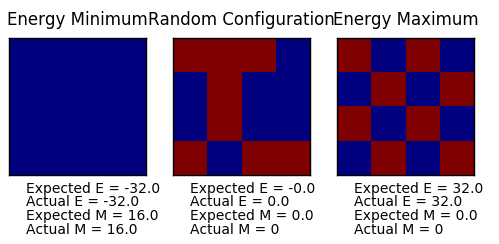
TASK: For the one dimensional case, there are two nearest neighbours with respect to the central atom. For 2- and 3-dimensional lattice systems, there are 4 and 6 respective neighbors. Overall, in a lattice with periodic boundary conditions, each lattice cell would have $2d$, nearest neighbours (where d=the number of dimensions). In the following model, it was assumed that the lattice was a 2-dimensional system.

$$\begin{gathered} Number \\ of \\ neighbouring \\ atoms \\ =2\times D \end{gathered}$$

$$\begin{gathered} where \\ D= \\ the \\ number \\ of \\ dimensions \end{gathered}$$

Using the equation in figure 1, the lowest energy state would correspond to a system where all the spins of the atoms are in the same state (either up or down): The factor of 1/2 is to account for the double counting of the interactions between the lattice atoms.

$$\begin{gathered} Energy \\ =(-\frac{1}{2}J \\ for \\ each \\ interaction)\times \left(the \\ number \\ of \\ neighbours\right)\times \left(number \\ of \\ atoms \\ in \\ lattice\right) \end{gathered}$$

$$\begin{gathered} Energy \\ =(-\frac{1}{2}J)\times \left(2D\right)\times \left(N\right) \end{gathered}$$

$$\begin{gathered} Energ{y}_{all \\ spins \\ aligned} \\ = \\ -DNJ \end{gathered}$$

TASK: As all the atoms have the same spin state, the multiplicity of the system is 1, there is only one way to arrange the system. This system would be present at a temperature of 0K.

$$\begin{gathered} \mathrm{\Omega } \\ = \\ 1 \end{gathered}$$

$$\begin{gathered} Entropy \\ = \\ {k}_B\ln 1 \end{gathered}$$

$$\begin{gathered} Entropy \\ = \\ 0 \end{gathered}$$

This result is consistent with the 3rd law of thermodynamics which states that "the entropy of a perfectly crystalline system is 0 at a temperature of 0K".

TASK: The change in spin from -1 to +1 for one of the cells can be thought of as two processes: Change from -1 to 0 and 0 to +1 spin For a ($$\begin{gathered} D=3, \\ N=1000, \\ ie \\ L=10 \end{gathered}$$) system in the lowest energy configuration, when one of the spins spontaneously change direction the energy change would correspond to:

Figure 3: Illustration of an Ising lattice in one (N=5), two (N=5x5), and three (N=5x5x5) dimensions. Red cells indicate the "up" spin", and blue cells indicate the "down" spin.

$$\begin{gathered} \mathrm{\Delta }Energy \\ to \\ change \\ to \\ 0 \\ spin=(\frac{1}{2}J\times 4D) \end{gathered}$$

$$\begin{gathered} \mathrm{\Delta }Energy \\ to \\ change \\ to \\ 0 \\ spin=(\frac{1}{2}J\times 4\times 3) \end{gathered}$$

$$\begin{gathered} \mathrm{\Delta }Energy \\ to \\ change \\ to \\ 0 \\ spin= \\ +6 \\ J \end{gathered}$$

$$\begin{gathered} \mathrm{\Delta }Energy \\ to \\ change \\ to \\ -1 \\ from \\ 1= \\ +6\times 2 \\ J \end{gathered}$$

$$\begin{gathered} \mathrm{\Delta }Energy \\ = \\ +12J \end{gathered}$$

The entropy of this system would increase, as there would be an increase in the number of ways to produce the state (increase in multiplicity).

$$\begin{gathered} \mathrm{\Omega } \\ = \\ 1.00\times 10^3 \end{gathered}$$

$$\begin{gathered} \mathrm{\Delta }Entropy \\ = \\ {k}_B\ln 1.00\times 10^3 \\ = \\ 9.54\times 10^{-23} \\ J \\ {K}^{-1} \end{gathered}$$

The magnetisation of the system is calculated by the sum of the parallel spins in the system. In the lowest energy configuration, where all the atoms in the lattice have the same direction of spin, the system would expect to have a maximum value of magnetisation. This corresponds to high ferromagnetic state.

$TotalMagnestisation=\sum _i{s}_i$

TASK: For figure 3, the magnetisation for the 1D and 2D case would be expected to be $$\begin{gathered} Total \\ Magnestisation \\ = \\ +1 \\ up \\ spin \end{gathered}$$, as the number of up spin states are greater than the number of down spin states. As there is no external magnetic field that is present in the system, the sign of magnetization is not significant.

TASK: For a ($$\begin{gathered} D=3, \\ N=1000, \\ ie \\ L=10 \end{gathered}$$) system where the atomic magnetic dipoles do not have sufficient energy to repel against their neighbours, it would be expected that the cells would be all aligned in the same direction. This would be most favourable in energetic terms and lead to a maximum magnetisation value of $$\begin{gathered} Total \\ Magnestisation=1000 \end{gathered}$$

Calculating the energy and magnetisation

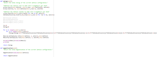
TASK: It was assumed that J=1.0 in the follow sections. When J>0 there is a energetic drive for the spins to align as this minimizes the energy of the system. The figure 4 below, presents the code that initally was used to calculate the energy and the magnetisation of the system. Please refer to the Accelerating Code section for the modified version of the script.

Energy

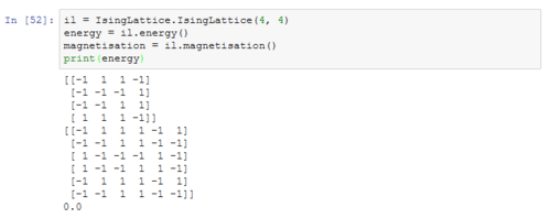
The figure 5 gives a visual illustration of the actions undertaken on the randomly generated original matrix. These actions were undertaken to ensure the final energy calculations of the matrix took into consideration the assumption of the periodic boundary conditions, and for the simplification of the energy calculations.

The 1st matrix that is printed in figure 5 is the original matrix random generated from [-1,1] states. The energy function takes copies of the 1st and last rows of the original matrix and creates a new matrix, where the copied last row of the original matrix, becomes the 1st row of the new matrix. Likewise, the 1st row of the original matrix becomes the last row of the new matrix. The original x matrix within this additional 'wall' of numbers was left untouched. This same operation was applied to the columns, such that a 6x6 matrix was formed. The calculation of the interaction energies was only applied to the original 4x4 matrix within the 'wall' of the copied values, using the equation in figure 1.

Magnetisation

As the matrix values represent the magnetic spin of atoms in a lattice, the values are restricted to [-1,1]. The sum of the spins values in the lattice is equal to the total magnetisation of the system; a simple sum(sum(x)) was applied to the matrix to return the total summation value. The model assumes that in the presence of no external magnetic field, the lattice can still generate a net magnetisation through the long range correlations.

molecule1	molecule1	molecule1
Figure 4: Method used to calculate the energy of the system	Figure 5: Initial 4x 4 matrix used to create a 6x6 matrix, which was used to calculate the total energy	Figure 6: Running the ILcheck.py script on the Ising Lattice model

TASK: The main engine of the model that initally was used to calculate the energy and magnetisation. Part of the IsingLatticeModel script.

def energy(self): "Return the total energy of the current lattice configuration." "Addition the lattice rows to take into 4 neighbours per atom" a=(np.insert(self.lattice, self.n_rows, self.lattice[0], axis=0)) b=(np.insert(a, 0, self.lattice[self.n_rows-1], axis=0)) "Addition the lattice columns to take into 4 neighbours per atom" c=(np.insert(b,self.n_cols,[row[0] for row in b], axis=1)) EditedLattice=(np.insert(c,0,[row[self.n_cols-1] for row in b], axis=1)) #print(self.lattice) #print(EditedLattice) #print(range(1,self.n_rows)) #print(range(1,self.n_cols)) J=1.0 Energy=0 for i in range(1,self.n_rows+1): for j in range(1,self.n_cols+1): Energy=Energy-0.5*J*EditedLattice[i][j]*EditedLattice[i][j+1]+-0.5*J*EditedLattice[i][j]*EditedLattice[i][j-1]+-0.5*J*EditedLattice[i][j]*EditedLattice[i+1][j]+-0.5*J*EditedLattice[i][j]*EditedLattice[i-1][j] return Energy def magnetisation(self): "Return the total magnetisation of the current lattice configuration." magnetisation=sum(sum(self.lattice)) return magnetisation

Introduction to Monte Carlo simulation

TASK: Please refer to the Accelerated Code section to see the modified IsingLattice code

TASK: Due to the spin up(+1) and spin down(-1) possibilities for each atom, there are a increasing number of configurations possible with the increasing number of atoms.

$$\begin{gathered} Configurations \\ Possible=2^N \end{gathered}$$

For a 100 spin system and computing power of $1\times 10^9$ calculations per second:

$$\begin{gathered} Processing \\ Time \\ =\frac{2^{100}}{1\times 10^9} \end{gathered}$$

$$\begin{gathered} Processing \\ time \\ for \\ one \\ value \\ of{⟨M⟩}_T \\ =1.27 \\ (2 \\ dp)\times 10^{21} \\ seconds \end{gathered}$$

molecule1	molecule1	molecule1	molecule1
Figure 7: Populated Monte Carlo and Statistics() functions	Figure 8: A single cycle of the Monte Carlo algorithm was implemented along with the statistics() function. The following quantities $<E>,<E^2>,<M>,<M^2>$, number of Monte Carlo steps that have elapsed, were returned by the function.	Figure 9: Plot of reduced energy per spin and reduced magnetisation per spin, against number Monte Carlo of steps	Figure 10: Plot of reduced energy per spin and reduced magnetisation per spin, against number Monte Carlo of steps - equilibrium system

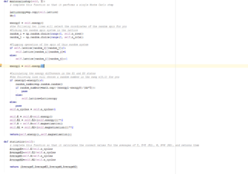
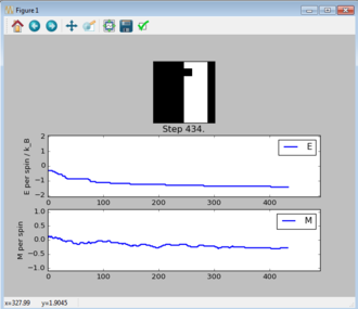
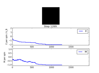
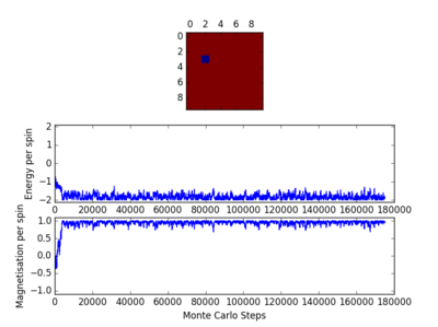
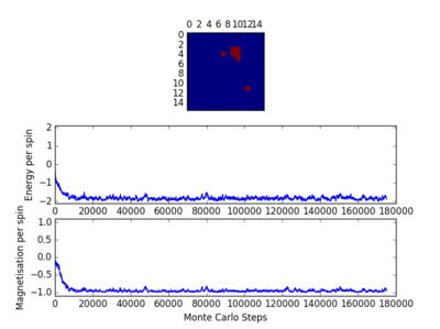
TASK: Figure 7 to 10 captures the development and testing of the montecarlocycle() and statistics() function. Figures 9 and 10 ultilised the ILanim.py script to animate a real time Monte Carlo simulation. Figure 9 presents the minimum energy and maximum magnetisation value of the system in equilibrium state (ie graphs of the energy and magnetisation per spin). It is expected that when $T<T_C$, there would be spontaneous magnetisation (i.e. $⟨M⟩\ne 0$) as the exchange and long range correlation effects would outweigh the thermal fluctuations, causing the neighboring atoms to favour aligning in the same direction. Above the $T_C$, the thermal energy in the system is sufficient to overcome any exchange and long range correlation effects.

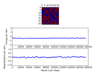
Figure 10 is a system in an equilibrium state.

$$\begin{gathered} Averaged \\ quantities: \end{gathered}$$

$<E>=-1.70271773681$

$<E^2>=3.02165944851$

$<M>=-0.800301970757$

$<M^2>=0.70215154164$

$$\begin{gathered} Number \\ of \\ Steps \\ =1274 \end{gathered}$$

Accelerating the code

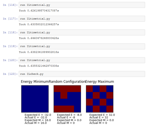
TASK: Using the script ILtimetrial.py, the time required to perform 2000 Monte Carlo steps in the IsingLattice.py script was calculated. On average the original code took:

$$\begin{gathered} Time \\ to \\ calculate \\ 2000 \\ steps= \\ 40.31605199s\pm \\ 0.271653419s \end{gathered}$$

The code was optimized using the roll() and multiply() functions. The original matrix was multiplied with the original matrix shifted by one unit in the x-axis and the original matrix shifted by one unit in the y-axis. This operation was able to capture the same neighbouring interactions as the previous code, but was more time efficient. On average the optimized code took:

$$\begin{gathered} Time \\ to \\ calculate \\ 2000 \\ steps= \\ 0.635318786s\pm \\ 0.009924127s \end{gathered}$$

molecule1	molecule1
Figure 11: Before Optimization of energy and magnetization code	Figure 12: After Optimization of energy and magnetization code

Optimized Ising Lattice Code

TASK: The main engine of the model that applies the Monte Carlo steps and calculates the energy and magnetisation of the system

import numpy as np import math as math class IsingLattice: E = 0.0 E2 = 0.0 M = 0.0 M2 = 0.0 NoIgnore = 160000 n_cycles = 0 def __init__(self, n_rows, n_cols): self.n_rows = n_rows self.n_cols = n_cols self.lattice = np.random.choice([-1,1], size=(n_rows, n_cols)) def energy(self): "Return the total energy of the current lattice configuration." J=1.0 Energy=0 NewL=np.multiply(np.roll(self.lattice, 1, axis=1),self.lattice) NewL2=np.multiply(np.roll(self.lattice, 1, axis=0),self.lattice) Energy=(sum(sum(NewL))+sum(sum(NewL2)))*-J return Energy def magnetisation(self): "Return the total magnetisation of the current lattice configuration." magnetisation=sum(sum(self.lattice)) return magnetisation def montecarlostep(self, T): # complete this function so that it performs a single Monte Carlo step latticecopy=np.copy(self.lattice) kb=1 energy0 = self.energy() #the following two lines will select the coordinates of the random spin for you #Picking the random spin system in the lattice random_i = np.random.choice(range(0, self.n_rows)) random_j = np.random.choice(range(0, self.n_cols)) #Flipping operation of the spin of this random system if self.lattice[random_i][random_j]<0: self.lattice[random_i][random_j]=1 else: self.lattice[random_i][random_j]=-1 energy1 = self.energy() #Calculating the energy difference in the E1 and E0 states #the following line will choose a random number in the rang e[0,1) for you if (energy1-energy0)>0: random_number=np.random.random() if random_number<=math.exp(-(energy1-energy0)/(kb*T)): pass else: self.lattice=latticecopy else: pass self.n_cycles = self.n_cycles+1 if self.n_cycles>=self.NoIgnore: self.E = self.E+self.energy() self.E2 = self.E2+(self.energy())**2 self.M = self.M+self.magnetisation() self.M2 = self.M2+(self.magnetisation())**2 else: self.E = 0 self.E2 = 0 self.M = 0 self.M2 = 0 return(self.energy(),self.magnetisation()) def statistics(self): # complete this function so that it calculates the correct values for the averages of E, E*E (E2), M, M*M (M2), and returns them if self.n_cycles>=self.NoIgnore: AverageE=self.E/(self.n_cycles-self.NoIgnore) AverageE2=self.E2/(self.n_cycles-self.NoIgnore) AverageM=self.M/(self.n_cycles-self.NoIgnore) AverageM2=self.M2/(self.n_cycles-self.NoIgnore) else: #if not above the number of cycles ignored, the system will ignore the value AverageE=0 AverageE2=0 AverageM=0 AverageM2=0 # take into consideration the ignored cycles in the printing of the number of steps undertaken return (AverageE,AverageE2,AverageM,AverageM2,(self.n_cycles-self.NoIgnore))

The effect of temperature

As the model starts from a random set of lattice spins, there is a certain number of steps required in order for the system to reach an energetic and magnetic thermal equilibrium. There are two main variables that effect this value:

• Lattice Size
• Temperature

Note: In each of the captions of the figures below, there is an approximated number of steps required to reach the equilibrium state

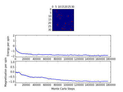
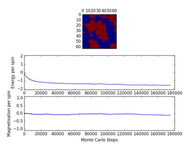
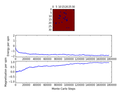
For figures 13 to 16 the temperature was kept constant at T=1.85, while the lattice size was increased. As seen below, with the increasing lattice sizes, the number of steps required to reach the equilibrium position increased. For example, the magnetisation and energy in the 10x10 lattice structure equilibrised <10000 steps, while in the 64x64 system the energy reached equilibrium at approx 160,000 steps.

Changing Lattice Size

molecule1	molecule1	molecule1	molecule1
Figure 13: Final state of the 10x10 lattice at T=1.85, runtime = 7500, equilibrium state<10000	Figure 14: Final state of the 16x16 lattice at T=1.85, runtime = 7500, equilibrium state≈10000	Figure 15: Final state of the 32x32 lattice at T=1.85, runtime = 30,000, equilibrium state≈120000	Figure 16: Final state of the 64x64 lattice at T=1.85, runtime = 50,000, equilibrium state≈140000

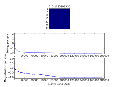
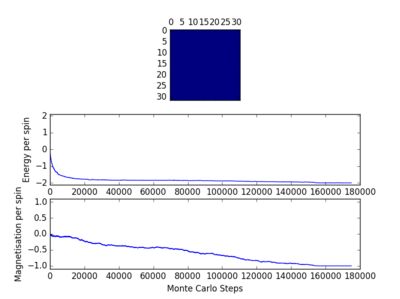
For figures 17 to 20, the lattice size was kept constant at 32x32, while the reduced temperatures were varied between T=0.25-5.0. With increasing temperatures of the system, the number of steps required to reach the equilibrium position in the system increased. For figure 20, T=5 is significantly greater than the Curie temperature for the system and thus the system reaches magnetic and energy equilibrium instantaneously as the thermal fluctuations eliminate all the correlation, enthaplic and entropic factors.

Changing Temperature

molecule1	molecule1	molecule1	molecule1
Figure 17: Final state of the 32x32 lattice at T=0.25, runtime = 175,000, equilibrium state≈90,000	Figure 18: Final state of the 32x32 lattice at T=0.80, runtime = 175,000, equilibrium state≈155,000	Figure 19: Final state of the 32x32 lattice at T=1.85, runtime = 175,000, equilibrium state≈160,000	Figure 20: Final state of the 32x32 lattice at T=5, runtime = 175,000, equilibrium state≈Immediately goes to equilibrium

TASK: It was found that for each lattice size and temperature, the system has a different number of cycles needed to obtain an equilibrium state. Based on the information above, for the worst case scenarios (T= approx 1.85 and very large lattice sizes eg 64x64), all the lattices reach an equilibrium by 160,000 steps. Therefore, the first 160,000 cycles of the Monte Carlo steps were chosen to be ignored in the calculation of the averages. This result led to the average values of magnetisation and energy having greater magnitudes and more accurate values for approximating the equilibrium system. A greater number of steps could have been ignored, and this may have lead to increased accuracy in the calculation of the variables, however in terms of the computational time required to calculate the these variables (eg for runtime=240,000) and the benefit obtained, it was decided that an optimal value of steps to ignore was 160,000.

The Ising Lattice script model no longer considers the energy and magnetisation values for the steps up to 160,000 ie until the system reaches an equilibrium point.

$$\begin{gathered} Averaged \\ quantities: \end{gathered}$$

$<E>=-1.99620390625$

$<E^2>=3.98527241211$

$<M>=0.999049609375$

$<M^2>=0.998119226074$

$$\begin{gathered} Number \\ of \\ steps \\ set \\ =240,000 \end{gathered}$$

Running over a range of temperatures/Scaling the System Size

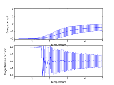
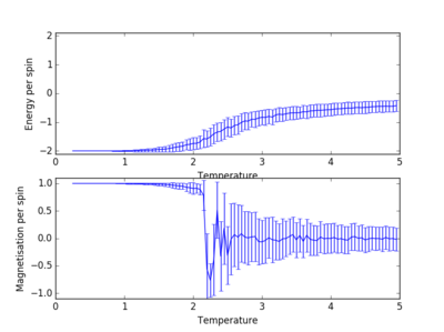
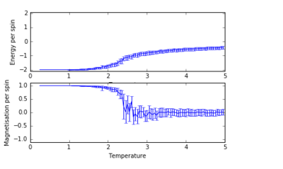
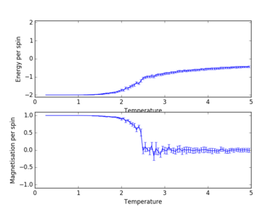
TASK: Using the ILtemperaturerange.py script, the average energy and magnetisation was plotted against the reduced temperature. Taking into account the 160,000 ignored simulations, the runtime was set to 240,000 and the dt steps adjusted to a lower value of 0.05 over a temperature range from T=0.25-5.0. This allowed the fine details of the fluctuations in energy and magnetisation for the system to be captured. The error bars at each temperature point, are calculated using the fluctuations in values from the runs conducted. The variability originates from the variations that occur in the $k_{B}T$.

molecule1	molecule1	molecule1	molecule1
Figure 21: Average energy and magnetisation simulations against temperature for the 4x4 lattice	Figure 22: TASK: Average energy and magnetisation simulations against temperature for the 8x8 lattice	Figure 23: Average energy and magnetisation simulations against temperature for the 16x16 lattice	Figure 24: Average energy and magnetisation simulations against temperature for the 32x32 lattice

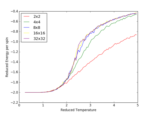
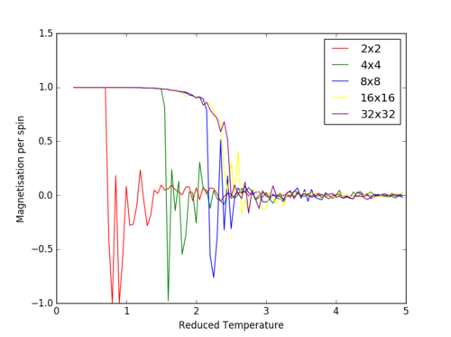
The $T_c$ Curie Temperature is the temperature at which the system undergoes a phase transition from an ordered to a disordered system and loses the net magnetization. The magnetisation changes rapidly at this point. Above the $T_c$ Curie Temperature, the changing of the spins from an ordered system to a completely disordered system – there is no energy penalty involved in this. In addition, there are long range correlation interactions present in the system which result a spin change, increasing the probability of triggering a spin change in another atom. Figure 25 captures the energy per spin against the reduced temperature. The energy rapdily increases upon reaching the Curie temperature; this graph resembles a $y=\sqrt[3]{|x|}$ function. With increasing lattice size, the energy per spin was observed to increase, with the 8x8,16x16 and 32x32 having very similar shapes.

The Curie temperature was observed to increase with increasing lattice sizes in figure 26, but contradicted the results of figure 25 in which the point of inflexion (steepest gradient for dE/dT) corresponds to the Curie temperature; the Curie temperature decrease with increasing lattice size. It is believed that for figure 26, the small size of the lattice caused inaccuracies in the simulations, due to the each lattice cell being so close to one another. The change in a spin of one cell in this lattice would dramatically increase the probability of the neighboring lattice cells changing spins. Furthermore, if the lattice cell spends half of its time in a total spin up state and the other half of its time in a total spin down state, the average of the system would end up being around zero.

TASK: Furthermore, the increased volatility around the $T_c$ Curie Temperature point decreases in significance with increasing lattice sizes (Figure 26). The temperature range at which the phase transition takes place, decreases with increasing lattice size. For a 32x32 system, the phase transition takes place almost instantly with insignificant volatility, while in the 4x4 system the transition takes place over approximately T=3 due to the fluctuation within the system. It is believed that for a lattice size of 16x16, the system is large enough to capture the long range fluctuations due to the sharp transition and the fluctuations observed.

molecule1	molecule1
Figure 25: Reduced energy per spin versus reduced temperature	Figure 26: Reduced magnetisation per spin versus reduced temperature

Running over a range of temperatures

TASK: Plotting of the average energy and magnetisation for each temperature, with error bars, for an 8x8 lattice

from IsingLattice import * from matplotlib import pylab as pl import numpy as np n_rows = 8 n_cols = 8 il = IsingLattice(n_rows, n_cols) il.lattice = np.ones((n_rows, n_cols)) spins = n_rows*n_cols runtime = 240000 times = range(runtime) temps = np.arange(0.25, 5.0, 0.05) #Empty arrays to be filled energies = [] magnetisations = [] energysq = [] magnetisationsq = [] stdenergy = [] stdmagnetisation=[] for t in temps: for i in times: if i % 100 == 0: print(t, i) energy, magnetisation = il.montecarlostep(t) aveE, aveE2, aveM, aveM2, n_cycles = il.statistics() energies.append(aveE) energysq.append(aveE2) magnetisations.append(aveM) magnetisationsq.append(aveM2) #reset the IL object for the next cycle il.E = 0.0 il.E2 = 0.0 il.M = 0.0 il.M2 = 0.0 il.n_cycles = 0 #Calculation in the energy and magnetisation errors of the system by calculating the Var(x) and then the standard deviations energyerror=np.array(energysq)-(np.array(energies)**2) magnetisationserror=np.array(magnetisationsq)-(np.array(magnetisations)**2) stdmagnetisation=np.sqrt(magnetisationserror) stdenergy=np.sqrt(energyerror) #Ploting figure and formatting issues fig = pl.figure() enerax = fig.add_subplot(2,1,1) enerax.set_ylabel("Energy per spin") enerax.set_xlabel("Temperature") enerax.set_ylim([-2.1, 2.1]) magax = fig.add_subplot(2,1,2) magax.set_ylabel("Magnetisation per spin") magax.set_xlabel("Temperature") magax.set_ylim([-1.1, 1.1]) #Addition of error bars for each of the temperature points run at enerax.errorbar(temps, np.array(energies)/spins,yerr=np.array(stdenergy)/spins) magax.errorbar(temps, np.array(magnetisations)/spins,yerr=np.array(stdmagnetisation)/spins) pl.show() final_data = np.column_stack((temps, energies, energysq, magnetisations, magnetisationsq,stdmagnetisation,stdenergy)) np.savetxt("32x32-larger dt.dat", final_data)

Scaling the System Size

TASK: The code below was used to plot energy and magnetisation per spin against temperature. Currently, it plots the energy but can be easily adapted for magnestism.

import matplotlib.pyplot as plt import numpy as np #Extracting the data from each data file and catergorising it into variables data2by2 = np.loadtxt("2x2.dat") spins2by2=4 temps2by2=data2by2[:,0] energies2by2=data2by2[:,1] energysq2by2=data2by2[:,2] magnetisations2by2=data2by2[:,3] magnetisationsq2by2=data2by2[:,4] data4by4 = np.loadtxt("4x4.dat") spins4by4=16 temps4by4=data4by4[:,0] energies4by4=data4by4[:,1] energysq4by4=data4by4[:,2] magnetisations4by4=data4by4[:,3] magnetisationsq4by4=data4by4[:,4] data8by8 = np.loadtxt("8x8.dat") spins8by8=64 temps8by8=data8by8[:,0] energies8by8=data8by8[:,1] energysq8by8=data8by8[:,2] magnetisations8by8=data8by8[:,3] magnetisationsq8by8=data8by8[:,4] data16by16 = np.loadtxt("16x16.dat") spins16by16=256 temps16by16=data16by16[:,0] energies16by16=data16by16[:,1] energysq16by16=data16by16[:,2] magnetisations16by16=data16by16[:,3] magnetisationsq16by16=data16by16[:,4] data32by32 = np.loadtxt("32x32.dat") temps32by32=data32by32[:,0] spins32by32=1024 energies32by32=data32by32[:,1] energysq32by32=data32by32[:,2] magnetisations32by32=data32by32[:,3] magnetisationsq32by32=data32by32[:,4] #graph curves colour selection plt.gca().set_color_cycle(['red', 'green', 'blue', 'yellow', 'purple']) #Calculation of the properties per spin and plotted plt.plot(temps2by2, energies2by2/spins2by2) plt.plot(temps4by4, energies4by4/spins4by4) plt.plot(temps8by8, energies8by8/spins8by8) plt.plot(temps16by16, energies16by16/spins16by16) plt.plot(temps32by32, energies32by32/spins32by32) plt.xlabel('Reduced Temperature') plt.ylabel('Reduced Energy per spin') plt.legend(['2x2', '4x4', '8x8', '16x16','32x32'], loc='upper right') plt.show() plt.savefig('test.jpg')

Determining the heat capacity

TASK: Proof of:

$C=\frac{\partial ⟨E⟩}{\partial T}$ = $\frac{\mathrm{V}\mathrm{a}\mathrm{r}[E]}{k_B{T}^2}$

LDS:

$C=\frac{\partial ⟨E⟩}{\partial T}$

$<E>=\frac{\sum _i^N{E}_i}{N}$ Or $<E>=\sum _i{E}_{i}P(E_i)$

$<E>=\frac{1}{\sum _i{e}^{-\frac{E_i}{k_{B}T}}}\sum _i(E_i{e}^{-\frac{E_i}{k_{B}T}})$

where $P(E_i)=\frac{1}{\sum _i{e}^{-\frac{E_i}{k_{B}T}}}\sum _i(e^{-\frac{E_i}{k_{B}T}})$

$C=\frac{\partial }{\partial T}\frac{\sum _i^N{E}_i}{N}=\frac{\partial }{\partial T}(\frac{1}{e^{-\frac{E_i}{k_{B}T}}}\sum _i(E_i{e}^{-\frac{E_i}{k_{B}T}}))$

Using the quotient rule:

$\frac{\partial ⟨E⟩}{\partial T}=\frac{(\sum _i{e}^{-\frac{E_i}{k_{B}T}})\times \sum _i(\frac{(E_i{)}^2}{k_B{T}^2}{e}^{-\frac{E_i}{k_{B}T}})-\sum _i(E_i{e}^{-\frac{E_i}{k_{B}T}})\times \sum _i(\frac{E_i}{k_B{T}^2}{e}^{-\frac{E_i}{k_{B}T}})}{\sum _i(e^{-\frac{E_i}{k_{B}T}}{)}^2}$

$\frac{\partial ⟨E⟩}{\partial T}=\frac{(\sum _i{e}^{-\frac{E_i}{k_{B}T}})\sum _i((E_i{)}^2{e}^{-\frac{E_i}{k_{B}T}})-\sum _i(E_i{e}^{-\frac{E_i}{k_{B}T}}{)}^2}{\sum _i(e^{-\frac{E_i}{k_{B}T}}{)}^2(k_B{T}^2)}$

$\frac{\partial ⟨E⟩}{\partial T}=\frac{1}{(k_B{T}^2)}(\frac{(\sum _i((E_i{)}^2{e}^{-\frac{E_i}{k_{B}T}})}{\sum _i(e^{-\frac{E_i}{k_{B}T}})}-\frac{\sum _i(E_i{e}^{-\frac{E_i}{k_{B}T}}{)}^2}{\sum _i(e^{-\frac{E_i}{k_{B}T}}{)}^2})$

$\frac{\partial ⟨E⟩}{\partial T}=\frac{\sum _i{E}_i^{2}P(E_i)-(\sum _i{E}_{i}P(E_i){)}^2}{(k_B{T}^2)}$

$\frac{\partial ⟨E⟩}{\partial T}=\frac{<E^2>-<E{>}^2}{k_B{T}^2}$

RDS:

$C=\frac{Var(E)}{k_B{T}^2}$

Calculating the heat capacity

Figure 26: TASK: Heat capacity versus temperature for the different lattice sizes

$C=\frac{\partial ⟨E⟩}{\partial T}$ = $\frac{\mathrm{V}\mathrm{a}\mathrm{r}[E]}{k_B{T}^2}$

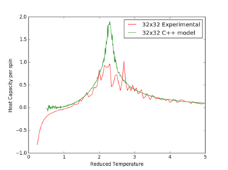
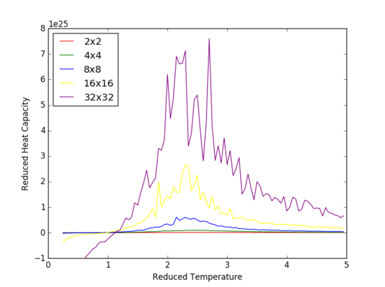
TASK: The increased detail and volatility around the curve at the $T_c$ Curie Temperature, is due to the lower value of dt=0.05 that was run in the 'Running over a range of temperatures' section. This section utilized the .dat files that were produced from the previous tasks. The heat capacity vs reduced temperature graph presents a strong peak in vicinity of the critical temperature, caused by the $C=\frac{\partial ⟨E⟩}{\partial T}$, the gradient of the energy per spin vs reduced temperature rapidly increasing near the Curie temperature. The point of inflexion in this graph (energy per spin vs reduced temperature) corresponds to the maxima peak observed in the heat capacity versus temperature graph. It is shown that with increasing array size, an increase in the peak amplitude is observed.

Calculating the heat capacity

TASK: Plot showing the heat capacity versus temperature for each of the lattice sizes from the previous section

import matplotlib.pyplot as plt import numpy as np #Load the data from the temperature range files and calculate the variance of each of the energies using the quoted formula data2by2 = np.loadtxt("2x2.dat") spins2by2=4 temps2by2=data2by2[:,0] Varenergies2by2=data2by2[:,2]-data2by2[:,1]**2 data4by4 = np.loadtxt("4x4.dat") spins4by4=16 temps4by4=data4by4[:,0] Varenergies4by4=data4by4[:,2]-data4by4[:,1]**2 data8by8 = np.loadtxt("8x8.dat") spins8by8=64 temps8by8=data8by8[:,0] Varenergies8by8=data8by8[:,2]-data8by8[:,1]**2 data16by16 = np.loadtxt("16x16.dat") spins16by16=256 temps16by16=data16by16[:,0] Varenergies16by16=data16by16[:,2]-data16by16[:,1]**2 data32by32 = np.loadtxt("32x32.dat") temps32by32=data32by32[:,0] spins32by32=1024 Varenergies32by32=data32by32[:,2]-data32by32[:,1]**2 plt.gca().set_color_cycle(['red', 'green', 'blue', 'yellow', 'purple']) #plotting of the Variance/kT2 against the reduced temperature plt.plot(temps2by2,Varenergies2by2/np.multiply(1.38064852e-23,temps2by2**2)) plt.plot(temps4by4, Varenergies4by4/np.multiply(1.38064852e-23,temps2by2**2)) plt.plot(temps8by8,Varenergies8by8/np.multiply(1.38064852e-23,temps2by2**2)) plt.plot(temps16by16, Varenergies16by16/np.multiply(1.38064852e-23,temps2by2**2)) plt.plot(temps32by32, Varenergies32by32/np.multiply(1.38064852e-23,temps2by2**2)) plt.xlim((0,5)) plt.ylim((-1E+25,0.8E+26)) plt.xlabel('Reduced Temperature') plt.ylabel('Reduced Heat Capacity') plt.legend(['2x2', '4x4', '8x8', '16x16','32x32'], loc='upper left') plt.show()

Locating the Curie temperature

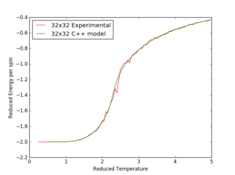
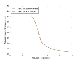
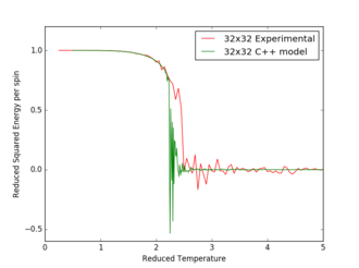
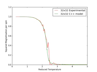
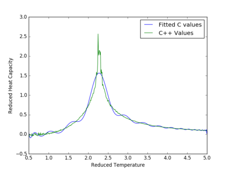
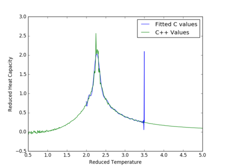
Figures 17 to 21 are the plots of the 32x32 lattice C++ data with the computational experimental data obtained for the $E,E^2,M,M^2,C$ per spin variables. The 32x32 lattice was used for the data comparison, as the volatility and error associated with the energy and magnetisation calculations for this lattice size was significantly lower than for the smaller arrays. A legend was added to the graphs to indicate the source of data. Overall, there is a good agreement between the C++ and the experimental data, however the C++ calculation method does show advantages in figure 31. The C++ data produces a pronounced peak, indicating a clear $T_C$, while the experimental data has large variability around this temperature point. This accuracy can be attributed to the large number of steps that the C++ data undertakes.

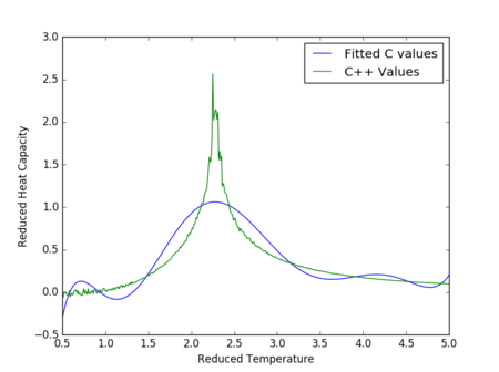
The figures 32-34 present the 'trial and error' method was applied to a 64x64 lattice, to produce the polynominal fit to the C++ data. It was found that a maximum polynominal value of 400 produced the best fit for the whole temperature range. However, due to the nature of the peak being very abrupt in the function, the polynominal fit function was unable to produce a satisfactory fit. When the temperature range of the polynominal fit function was reduced to the regions of the peak, the polynominal was able to produce a good fit (figure 34).

TASK:

molecule1	molecule1	molecule1	molecule1	molecule1
Figure 27: TASK: Plotting reduced energy per spin against reduced temperature	Figure 28: TASK: Plotting reduced energy squared per spin against reduced temperature	Figure 29: TASK: Plotting reduced magnetisation per spin against reduced temperature	Figure 30: TASK: Plotting reduced magnetisation squared per spin against reduced temperature	Figure 31: TASK: Plotting reduced heat capacity per spin against reduced temperature

Comparing the C++ data and the experimental data

TASK: For each lattice size, plotting the C++ data against experimental data. This current code is optimized for comparing the heat capacity values across the temperature range, but can be made to plot for $E,E^2,M,M^2,C$

import matplotlib.pyplot as plt import numpy as np #My experimental data, calculation of the variance of the energy to use in the equation for the heat capacity data32by32 = np.loadtxt("32x32.dat") spins32by32=32*32 temps32by32=data32by32[:,0] Varenergies32by32=data32by32[:,2]-data32by32[:,1]**2 #C++ data provided Cdata32by32 = np.loadtxt("32x32c++.dat") Cspins32by32=32*32 Ctemps32by32=Cdata32by32[:,0] Cenergies32by32=Cdata32by32[:,5] #print(Cenergies32by32) plt.gca().set_color_cycle(['red', 'green', 'blue', 'yellow', 'pink']) #calculation of the actual heat capacity ie mulitplied by kb + plotting the data on the same graph plt.plot(temps32by32, (1.38064852e-23*Varenergies32by32/np.multiply(1.38064852e-23,temps32by32**2))/spins32by32) plt.plot(Ctemps32by32,Cenergies32by32) plt.xlabel('Reduced Temperature') plt.ylabel('Heat Capacity per spin') plt.legend(['32x32 Experimental', '32x32 C++ model'], loc='upper right') plt.show()

Comparing C++ data and experimental data + polynominal fitting

TASK: A script to read the data from a particular file, and plot C vs T, as well as a fitted polynomial. The 400 degree polynomial was found to be the best fit without restricting the temperature ranges. Figures 32-33

TASK: Modified version of the previous script to fit the polynomial to the peak of the heat capacity ie restricting the temperature range figures 34

molecule1	molecule1	molecule1
Figure 32: TASK: Polynomial 8 for a 64x64 lattice	Figure 33: TASK: Polynomial 400 for a 64x64 lattice	Figure 34: TASK: Polynomial 400 for a 64x64 lattice restricted to fit between T2 to T3.5

import matplotlib.pyplot as plt import numpy as np #List for the values of the maximum heat capacity and temperature to go into Temperature=[] HeatCapacity=[] length=[2,4,8,16,32,64] name=["2x2c++","4x4c++","8x8c++","16x16c++","32x32c++","64x64c++"] #Loop to export data intp python from various c++ data files for i in name: naming= i+".dat" data = np.loadtxt(str(naming)) #assume data is now a 2D array containing two columns, T and C T = data[:,0] #get the first column C = data[:,5] # get the 6th column #The region which the polynominal will fit to Tmin = 1.5 Tmax = 4.0 #Restricting the peak picking to the temeprature peak region due to peaks at the edge of boundaries #Restricting Tmin and Tmax to other values if produces a better fit to the data if i=="2x2c++": Tminforpeak = 1.5 Tmaxforpeak = 3.0 elif i=="4x4c++": Tminforpeak = 1.7 Tmaxforpeak = 3.3 elif i=="8x8c++": Tminforpeak = 1.8 Tmaxforpeak = 3.3 elif i=="16x16c++": Tmin = 1.5 Tmax = 2.9 Tminforpeak = 1.5 Tmaxforpeak = 2.8 elif i=="32x32c++": Tmin = 1.5 Tmax = 2.8 Tminforpeak = 1.5 Tmaxforpeak = 2.7 else: Tmin = 1.5 Tmax = 2.75 Tminforpeak = 1.5 Tmaxforpeak = 2.7 selection = np.logical_and(T >=Tmin, T <= Tmax) #choose only those rows where both conditions are true peak_T_values = T[selection] peak_C_values = C[selection] #first we fit the polynomial to the data fit = np.polyfit(peak_T_values, peak_C_values, 400) # fit a third order polynomial #now we generate interpolated values of the fitted polynomial over the range of our function T_range = np.linspace(Tminforpeak , Tmaxforpeak, 1000) #generate 1000 evenly spaced points between T_min and T_max fitted_C_values = np.polyval(fit, T_range) # use the fit object to generate the corresponding values of C #print(T) Cmax = np.max(fitted_C_values) Tmax = T_range[fitted_C_values == Cmax] #Exporting the Heat Capacity maximum, temperature value and the corresponding lattice size to a .dat file Temperature.append(Tmax) HeatCapacity.append(Cmax) final_data = np.column_stack((np.array(length),np.array(Temperature), np.array(HeatCapacity))) np.savetxt("Heat Capacity Ising Model.dat", final_data)

Finding the peak in C

TASK:

$T_{C,L}=\frac{A}{L}+T_{C,\mathrm{\infty }}$

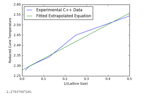
Using the equation above, the 1/(lattice length) was plotted against the reduced temperature. The resulting linear relationship was then extrapolated and calculated at T=0; corresponds to the value of $T_{C,\mathrm{\infty }}$. This was compared with Onsager(1944) literature values and had very good agreement.

The major sources of error are due to the assumptions made in the model:

• The noise at the peak value creates uncertainty in the plot fitting
• Assumption that the relationship in figure 35 is linear
• Required to extrapolation data for T=0 - uncertainty in what the actual data would be in this region
• There are more than 4 nearest neighbours around a lattice cell; the longer range of interactions are not considered

$T_{C,\mathrm{\infty }}(C^{++}experimental)=2.27837987241$

$T_{C,\mathrm{\infty }}(literaturereports)=2.27$

molecule1	molecule1
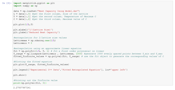
Figure 35: Plot of the reduced temperature against 1/(lattice length)	Figure 36: Code used to produce Figure 35, in addition to the extrapolation of the $T_{C,\mathrm{\infty }}$

TASK: A plot that uses the scaling relation to determine $T_{C,\mathrm{\infty }}$

import matplotlib.pyplot as plt import numpy as np data = np.loadtxt("Heat Capacity Ising Model.dat") L = data[:,0] #get the first column, Size of the Lattice T = data[:,1] #get the second column, Temperature of Maximum C C = data[:,2] #get the third column, Maximum value of C plt.plot(1/L,T) plt.xlabel('1/(Lattice Size)') plt.ylabel('Reduced Heat Capacity') #extrapolation for 1/lattice size values Latticemax = np.ndarray.max(1/L) Latticemin = 0 #extrapolation using an approximate linear equation fit = np.polyfit(1/L, T, 1) # fit a first order polynomial ie linear T_range = np.linspace(Latticemin , Latticemax, 1000) #generate 1000 evenly spaced points between T_min and T_max fitted_Tinfinite_values = np.polyval(fit, T_range) # use the fit object to generate the corresponding values of C #Plotting the fitted equation plt.plot(T_range, fitted_Tinfinite_values) plt.legend(['Experimental C++ Data','Fitted Extrapolated Equation'], loc='upper left') plt.show() #Printing out the Tinfinite value print(np.polyval(fit, 0))