Rep:MgO:mmn115

Abstract

In this experiment, the thermal expansion coefficient ($\alpha$) for the MgO crystal lattice was computed using the Quasi-Harmonic approximation (QHA) and Molecular Dynamics (MD) methods. The 'k' grid size which is a reasonable approximation of an infinite lattice was found to be 18x18x81. The results obtained with these two methods were then compared. It was found that for low temperatures (100-400K), the QHA works better than MD, as it considers the zero-point energy. The $\alpha$ values obtained for QHA and MD were compared with experimental literature values: $\alpha =14.60\times 10^{-6}{K}^{-1}$ for QHA, $\alpha =18.68\times 10^{-6}{K}^{-1}$ for MD and $\alpha =10.42-12.02\times 10^{-6}{K}^{-1}$ in literature . For higher temperatures (400-2100 K), MD fits the expected linear trend more accurately and is therefore a better approximation, as it considers the anharmonicity.

Introduction

MgO structure

MgO adopts a crystal structure of rock-salt. There are three types of cells which must be considered for MgO: conventional, primitive and supercell.

The conventional cell (Figure 1) adopts a cubic structure where a=b=c, a, b and c being the lattice parameters. It is an fcc lattice of Mg²⁺ ions with O^2- ions occupying all the octahedral holes or vice versa. The internal angle is equal to 90 degrees and there are 8 ions in the cell: 4 Mg²⁺ and 4 O^2- .

The structure can also be represented using a primitive cell (Figure 2). In the primitive cell, there are 4 ions in total: 2 Mg²⁺ and 2 O^2-.The lattice parameters a=b=c and the internal angle is equal to 60 degrees, as the structure is a rhombohedron. An integer multiple of the primitive cell makes up the conventional cell.

Another way to represent the crystal structure of MgO is using a supercell (Figure 3). A supercell is a repeating unit of a conventional cell , where a=b=c, and, in this experiment, the lattice parameter is equal to twice the lattice parameter of the conventional cell, ie. the conventional cell is 'doubled' in x,y and z directions. The internal angle is 90 degrees. In this investigation, a supercell consisting of 32 MgO units will be used (64 ions in total, half Mg²⁺ and half O^2-).

The primitive cells are used for the calculations based on the quasi-harmonic approximation, whereas for molecular dynamics simulations the supercell is used.

Furthermore, it is important to note that real crystal lattices contain defects. In this investigation, all the calculations are based on the assumption that the lattice is perfect, ie. contains no defects.

Figure 1. Conventional cell model

Figure 2. Primitive cell model

Figure 3. Supercell model

Quasi Harmonic approximation

Let us first consider the harmonic approximation and why it cannot be used to determine the thermal expansion of a crystal.

In the harmonic oscillator, when a system of mass m experiences a displacement x from the equilibrium position, it will experience a force F which will restore it to its original position:

Equation 1

where F is the restoring force, k is the force constant and x is the displacement. Consider for example a mass on a spring, which is a classic example of the harmonic oscillator.

The motion of the system of mass m is described by the following equation:

Equation 2

where x is the displacement from equilibrium at time t, A is the amplitude, phi is the phase which determines the starting point of the cosine wave and ω is the frequency which is defined by:

Equation 3

where T is the period and m is the mass. Therefore, clearly, it is a periodic function.

The potential of the system is expressed by:

Equation 4

where V is the potential, k is the force constant and x is the displacement. From the equation it can be seen that the potential energy curve is a parabola. Some thermodynamic properties, such as temperature dependence of entropy or Helmholtz free energy can be computed using the harmonic approximation. The harmonic approximation is also useful to compute dispersion curves and phonon density of states. However, other properties, such as thermal expansion or Helmholtz free energy as a function of temperature and pressure need to go beyond the harmonic approximation .

This is because in the harmonic approximation the equilibrium position of the nuclei is fixed and it does not vary with temperature.Therefore, as the temperature is varied, the lattice parameters, and the volume, would not change, which defeats the purpose of the experiment. The thermal expansion coefficient cannot be calculated using the harmonic approximation, because the system is not allowed to change volume. T

Furthermore, at higher temperatures, the molecules or atoms will dissociate and the potential will go to infinity. The harmonic oscillator does not take into account the dissociation, the anharmonicity, and therefore breaks down at higher temperatures.

Helmholtz free energy is temperature dependent. As the equilibrium position is always that with the lowest free energy, this suggests that it may be possible to monitor the temperature dependence on volume of the crystal by monitoring the lowest free energy. The quasi-harmonic approximation (QHA) assumes that the anharmonicity is only related to thermal expansion. Therefore, the temperature dependence of the phonon energies arises from the dependence on crystal structure and volume . The QHA introduces dependence of volume on phonon frequencies, at the same time retaining the harmonic expression for the free energy . As a result, the following expression is obtained:

Equation 5

where ω is the frequency, j is the number of branches, k is the number of k points, F is the free energy, k_b is the Boltzmann constant, T is the temperature and E₀ is the internal energy. The second term represents the zero-point energy and the third term corresponds to the vibrational entropic contribution.

Therefore, the QHA can be used to calculate the thermal expansion coefficient.

Molecular dynamics

Molecular Dynamics (MD) is a computational modelling method which studies the physical movement of atoms and molecules . Basically, using the energy function, the force experienced by an atom at a given time and given position can be calculated, provided that the position of the other atoms is known. It uses an algorithm in which the time is divided into discrete time steps. At each time step, the forces acting on each atom are computed. Next, the atom is moved by a bit and the position and velocity of each atom is updated by numerical solving of Newton's laws of motion . The information from all the time steps is then collected to compute the classical trajectory. What is important to note is that, unlike QHA, MD includes anharmonic interactions.

Certain limitations of the method include: the requirement for short timescales (femtoseconds), which can be a problem in studying, for example, proteins, as structural changes in proteins take longer; force fields are just approximations and are still quite inaccurate; covalent bonds cannot break and form during the simulations .

Popular applications of the MD method include determining where drug molecules bind and how they exert their effect, determining functional mechanims for proteins or understanding the process of protein folding .

Thermal expansion coefficient

Thermal expansion is when a material fractionally increases its size in response to applied temperature. In the case of MgO, which is a 3D structure, the thermal expansion can be monitored by looking at the change in lattice parameter and/or volume.

As temperature is increased, the energy of the molecules increases, their thermal motion increases and so they populate higher energy levels. As they move to higher energy states on the potential energy surface, on average, they will spend more time away from the equilibrium position, so the internuclear distance increases, resulting in a volume increase. Furthermore, the entropic advantage associated with lower frequencies and hence larger volume outweighs the enthalpic gain associated with minimizing the volume .

The coefficient of thermal expansion is the ratio of the fractional change of the size of the material to the change in temperature . It is given by the following equation:

Equation 6

where alpha is the thermal expansion coefficient, V is the volume, T is the temperature and V_i is the initial volume.

Solids will tend to retain their shape upon expansion (if not constrained) and so a linear expansion coefficient is expected.

Thermal expansion has various real-life applications. For example, consider a glass jar with a metal lid. If the lid is too tight, the jar and the lid can be put under running hot water in order to make it less tight. The lid will let go and the glass jar is not deformed in the process. This is because metals tend to have higher thermal expansion coefficients than glass, which means that under hot water the lid will expand, leaving the glass unchanged. Another example is a mercury thermometer. Mercury has a larger thermal expansion coefficient than the glass in which it is placed. As a result, mercury rises and falls in response to temperature changes. Finally, thermal expansion coefficients are also used in engineering. Expansion joints are placed in bridges. During the day, the bridge expands due to heat from the sun, so the expansion joints move away from each other. At night, when the bridge cools down, it contracts, and the joints move towards each other. As a result, the bridge is not constrained, and can expand and contract in response to temperature changes .

Reciprocal space

The structure of MgO is periodic and therefore can be represented both in real space and in reciprocal space. In real space, position vectors, r are used, whereas in reciprocal space the wavevector k is defining. The reciprocal lattice, located in reciprocal space, is formed by performing a Fourier transform on the original lattice in real space, the Bravais lattice. In the case of a cubic Bravais lattice, with lattice constant a, the reciprocal lattice is cubic as well with lattice parameter, a*, equal to:

Equation 7

This has important implications for the size of the cell used for calculations.

For QHA, reciprocal space is used. Therefore, all the vibrations of an infinite lattice can be represented in a finite space, so a primitive cell is used.

For MD, real space is used. All the atoms are moved, so in order for the method to be an accurate representation of the random movement of atoms, a bigger cell is needed. Hence, a supercell is used.

Method

For the simulations, the General Utility Lattice Program (GULP) was used as the molecular modelling code. The package DLV 3DView was used to visualise the structure and its properties. It was ensured that the option 'include shells' is not selected. 'ionic.lib' was selected in the GULP potential parameters panel.

Calculating the phonon modes of MgO

The phonon dispersion curve was plotted using the Execute GULP panel and selecting phonon dispersion. The number of phonons computed along this path was set to 50.

Next, the phonon density of states (DOS) was computed using the Execute GULP panel and selecting phonon DOS. The shrinking factors were initially set to A=1, B=1 and C=1, ie. a grid of size 1x1x1. The shrinking factors were then increased to A=B=C=2, A=B=C=4, A=B=C=6 .... up to A=B=C=24, going up in steps of two and always keeping A=B=C. This was done in order to determine the minimum grid size which would be a reasonable approximation of the density of states. The grid was found to be 18x18x18. The phonon DOS for the 1x1x1 grid was found to correspond to the L point on the dispersion curve.

Computing the free energy - the harmonic approximation

The free energy was calculated for various grid sizes using the quasi-harmonic approximation. Initially, the shrinking factors were set to A=B=C=1, temperature T=300 K and pressure 0 GPa. Phonon DOS was executed from the Execute GULP panel and the free energy for the system was reported. The procedure was then repeated but increasing grid size to the same values as before (A=B=C=1, 2, 4, 6, 8, 10, 12, 14, 16, 18, 20, 22, 24), keeping the temperature and pressure constant. From the 18x18x18 grid, the free energy started converging, so this confirmed the estimation from before that this grid size is a reasonable approximation of the free energy of the infinite lattice.

The thermal expansion of MgO

The free energy was then calculated for various temperatures using the quasi-harmonic approximation. The grid size was chosen to be 18x18x18, as from previous calculations it was determined as the minimal grid size which is a reasonable approximation of the infinite grid. Initially, the temperature was set to 0 K. The optimisation was performed using the Execute GULP panel and selecting 'photon DOS' and 'optimise Gibbs free energy'. The procedure was then repeated but changing the temperature from 0 K to 2900 K in steps of 100 K.

The log file was then used to extract the free energy and primitive cell volume. In order to obtain the lattice parameter, the primitive cell volume was multiplied by 4 to give the conventional cell volume. Next a cube root of the result was taken to give the lattice parameter.

Temperature vs volume were plotted and the slope of the curve and the initial volume were used to calculate the thermal expansion coefficient using Equation 6.

Molecular Dynamics

The volume was then calculated for various temperatures using the Molecular Dynamics (MD) method. Using the Execute GULP panel, the number of particles (N), pressure (P) and temperature (T) were fixed, allowing the volume to vary (NPT ensemble). The time-step was set to 1.0 femtosecond, equilibration steps to 500, production steps to 100, sampling steps to 5 and trajectory steps to 5. The initial temperature was set to 0 K, however, this did not work. The temperature was changed to 100 K and GULP was executed. The procedure was then repeated while varying the temperature in steps of 100 K all the way up to 2900 K.

In MD, a supercell is used containing 32 MgO units. Therefore, to obtain the conventional cell volume, the volume of the supercell extracted from the log file was divided by 8. The volume of the conventional cell was then cube rooted to give the lattice parameter.

Temperature vs volume were plotted and, as before, the slope of the curve and the initial volume were used to calculate the thermal expansion coefficient using Equation 6.

Results and discussion

Calculating phonon modes of MgO

The dispersion curve for a single k-point and the phonon DOS for the 1x1x1 grid were plotted:

Figure 4. Phonon DOS for 1x1x1 grid

Figure 5. Dispersion curve for a single k-point

For the phonon DOS of the 1x1x1 grid, there are four narrow peaks at around the following frequencies: 290, 350, 690 and 800 cm^-1. In the dispersion curve, a k-point through which 4 curves pass at frequencies corresponding to the ones in the phonon DOS is the L point. Furthermore, in the DOS, the two peaks at lower frequencies have double the intensity of the two peaks at higher frequencies. This suggests that the two peaks at lower frequencies correspond to two doubly degenerate vibrational modes. This gives a total of 6 bands. However, as two are doubly degenerate, they overlap and only four peaks are present. When looking at the L point on the dispersion curve, it is clear that there are two branches crossing each other at a frequency of around 290 cm-1 and two branches crossing each other at a frequency of around 350 cm^-1. This again confirms that the phonon DOS 1x1x1 grid was computed for the L-point.

This is further confirmed by the Log File in which it is given that the Brillouin zone sampling points are the following: x=0.50, y=0.50 and z=0.50. These correspond to the L point on the dispersion curve, which confirms that the DOS for 1x1x1 grid was plotted for the L point. Furthermore, in the Log File the frequencies of the vibrations are given as: 288.49, 288.49, 351.76, 351.76, 676.23 and 818.82 cm^-1. This confirms the observation made by visual inspection that the two peaks at lower frequencies are doubly degenerate.

The phonon density of states (DOS) for different grid sizes is shown below. As the grid size increases, the number of vibrational bands increases and the range of frequencies over which they appear increases. This is because with increasing grid size the number of sampled k-points increases, which in turn increases the number of phonons. Previously, there were four discrete, sharp peaks. Now, the peak becomes broader and more continuous. This is shown below:

• 
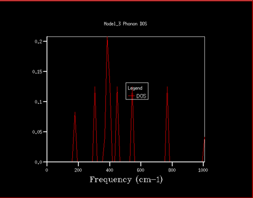  Figure 6. Phonon DOS for 2x2x2 grid
• 
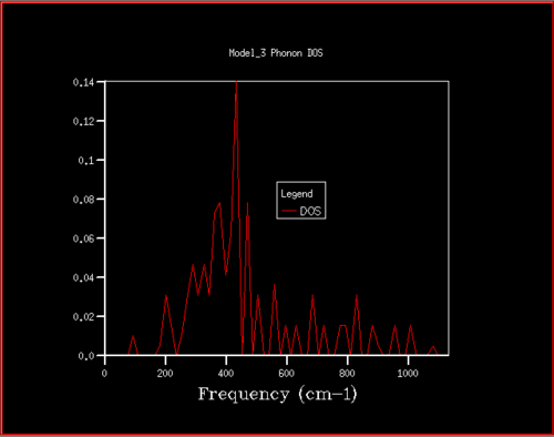  Figure 7. Phonon DOS for 4x4x4 grid
• 
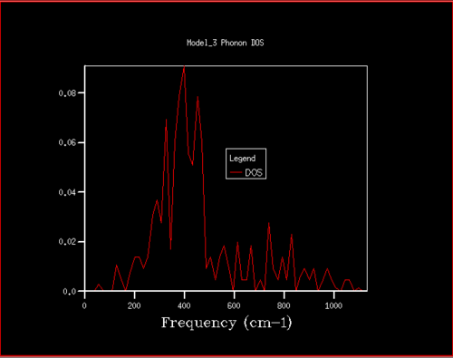  Figure 8. Phonon DOS for6x6x6 grid
• 
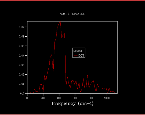  Figure 9. Phonon DOS for 8x8x8 grid
• 
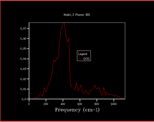  Figure 10. Phonon DOS for 10x10x10 grid
• 
  Figure 11. Phonon DOS for 12x12x12 grid
• 
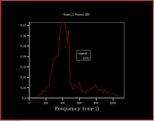  Figure 12. Phonon DOS for 14x14x14 grid
• 
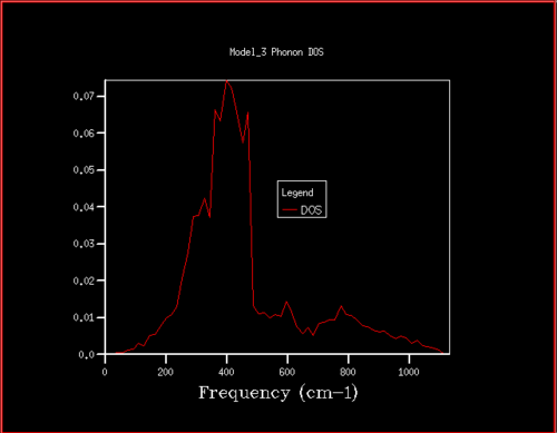  Figure 13. Phonon DOS for 16x16x16 grid
• 
  Figure 14. Phonon DOS for 18x18x18 grid
• 
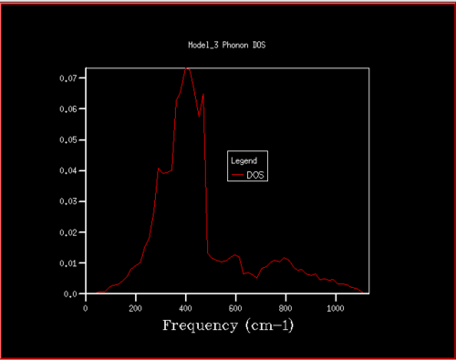  Figure 15. Phonon DOS for 20x20x20 grid
• 
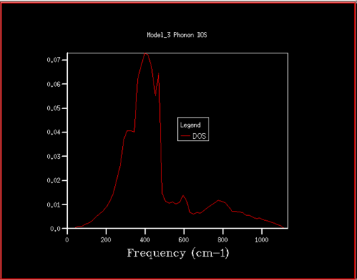  Figure 16. Phonon DOS for 22x22x22 grid
• 
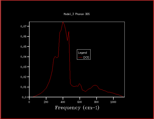  Figure 17. Phonon DOS for 24x24x24 grid

Starting at a grid size of around 18x18x18, the phonon DOS stops changing as much and the peak at around 400 cm^-1 becomes constant. It can therefore be assumed that the grid of size 18 is the minimum reasonable approximation for the density of states, as DOS changes from size 18 to size infinity will be very small.

For grid sizes smaller than 18, the DOS shows peaks at less frequencies and the peaks are narrower, sharper. For grid sizes larger than 18 the DOS resembles the DOS for grid size 18: the spectrum is more continuous and there is a large broad peak at a frequency of around 400 cm^-1. This observation can be explained by looking at the dispersion curve. In the frequency range of around 400 cm^-1, the curves are flatter than in other frequency ranges (compare to for example the steep, almost quadratic, slope of curves at 1000 cm^-1). As a result, there are many k-points in the 400 cm^-1 frequency range. This gives a large density of states in the 400 cm^-1 region which is reflected in the phonon DOS. Also, the two peaks at lower frequencies have larger intensities than the other two. This is due to the degeneracy of states.

The relationship between DOS and dispersion curves becomes more clear now. The DOS sums all the k-points at a particular frequency in the dispersion curve.

As the size of the ion decreases, the lattice parameter 'a' decreases as well. Therefore, from Equation 7, a* will increase which implies larger reciprocal space. As a result, more k-points are needed to achieve the same accuracy.

Consider CaO. Ca²⁺ is in period 4 whereas Mg²⁺ is in period 3. This means that the calcium ion will be larger, a will increase, a* will decrease, which means smaller reciprocal space so less k points are needed. Therefore, a smaller grid can be used to obtain similar accuracy as for the 18x18x18 grid for MgO. But because the difference in size between Ca²⁺ and Mg²⁺ is not very significant, 18x18x18 grid would probably work as well.

Zeolites are very large aluminosilicates. a is large, so a* will decrease significantly, giving a very small reciprocal space so less k-points are needed. In order to reduce computational cost and timescale of the simulations, a smaller grid should be used.

Li⁺, on the other hand, is a smaller ion than Mg²⁺ or O^2-. Therefore, following the analogy from before, it will have a smaller a, hence bigger a* and bigger reciprocal space. More k-points are needed to achieve good accuracy so a larger grid size should be used.

Computing the Free Energy - the harmonic approximation

The variation of free energy with grid size was monitored and the following result was obtained:

Table 1. Variation of free energy with grid size

grid size	free energy (eV)
1x1x1	-40.930301
2x2x2	-40.926609
4x4x4	-40.926609
6x6x6	-40.926471
8x8x8	-40.926410
10x10x10	-40.926480
12x12x12	-40.926481
14x14x14	-40.926482
16x16x16	-40.926482
18x18x18	-40.926483
20x20x20	-40.926483
22x22x22	-40.926483
24x24x24	-40.926483

At a grid size of 18 (18x18x18), the free energy starts converging and for the following three grid sizes it remains constant and equal to -40.926483 eV. With an increasing grid size, the accuracy would increase insignificantly but the computational cost associated with longer runs and more computational power required is larger than the gained accuracy. Therefore, it is reasonable to assume that the grid size of 18 is a good approximation of the infinite lattice and it will be used further calculations.

As the grid size increases, the number of k-points increases. This means that the accuracy of the calculations increases as well, because more k-points are sampled.

In order to decide which grid size would be appropriate for calculations accurate to 1 meV, 0.5 meV and 0.1 meV per cell, the deviation of the free energy value for each grid from the converged value must be calculated:

Table 2. Deviation from converged value of free energy of each grid size

grid size	deviation from converged value (eV)
1x1x1	0.003818
2x2x2	0.000126
4x4x4	0.000126
6x6x6	0.000012
8x8x8	0.000073
10x10x10	0.000003
12x12x12	0.000002
14x14x14	0.000001
16x16x16	0.000001
18x18x18	0
20x20x20	0
22x22x22	0
24x24x24	0

To obtain an accuracy of 1 meV, it is enough to use the 2x2x2 grid. To obtain an accuracy of 0.5 meV, the 2x2x2 grid can also be used. To obtain an accuracy of 0.1 meV, the 6x6x6 cell must be used. Note that, of course, larger grids can always be used to improve the accuracy. However, the larger the grid, the larger the computational cost associated with running the simulation and the gain in accuracy is not significant. Therefore, when looking for an 'appropriate' grid size, a compromise between accuracy and computational cost must be reached.

Thermal Expansion of MgO

Temperature vs free energy

The temperature was plotted vs Helmholtz free energy using the quasi-harmonic approximation and a linear fit was performed. The following graph was obtained:

The trend can be explained using the following equation:

$A=U-TS$

Equation 8

where A is the Helmholtz free energy, U is the internal energy, T is temperature and S is entropy. Therefore, it is expected that the free energy will decrease linearly with increasing temperature.

However, it can be seen that there are two parts of the graph. The first part is in the range 0-300 K and deviates from the linear trendline quite significantly. The slope is quite flat, the free energy does not change much with temperature and the free energy seems to be almost temperature-independent. As we go to temperatures above 300 K, the second part of the graph, the slope of the curve increases, the behaviour becomes more linear and the temperature-free energy dependence becomes more significant. The range 400-2900 K follows the equation above better.

Figure 19. Graph of the temperature vs Helmholtz free energy, calculated based on the quasi harmonic approximation, shown for the temperature range 400-2900K

This can be explained by looking at Equation 5 for free energy in the introduction:

At low T, the contribution of the last term (which is temperature dependent) to the free energy is negligible. The zero-point energy is the major contribution to the equation (second term) and it is independent of the temperature. As temperature increases, the third term starts to be more dominating so the behaviour of the curve changes, free energy becomes more dependent on the temperature so the curve becomes steeper.

Temperature vs lattice constant

Next, the lattice parameter was plotted against temperature and a line of best fit was computed. The quasi harmonic approximation was used for the calculations.

Figure 20. Graph of temperature vs lattice parameter calculated using QHA

The temperature vs volume of conventional cell graph was also plotted, together with the linear trendline.

Figure 21. Graph of temperature vs volume calculated using QHA

Again, by looking at Figure 21 and the linear fit, three parts of the graph can be distinguished.

Part 1 is the temperature range 100-400 K, where the slope of the linear fit is quite flat and the volume does not change very much with temperature. This can be explained by looking at the following equation for free energy:

$A=U-TS$

Equation 9

where A is the free energy, U is the internal energy, T is temperature and S is entropy. The change in internal energy, dU, can also be written as:

$dU=TdS-pdV$

Equation 10

where V is the volume and p is pressure. It is now clear that internal energy depends on volume, so free energy depends on volume as well:

$dA=-SdT-pdV$

Equation 11

Therefore, the trend for the T vs volume graph is the same as the trend for the T vs free energy graph, and can be explained using the same arguments as above (large contribution of zero-point energy to free energy at low T).

As the temperature increases, we get to part two (400-2100 K), where the slope of the line increases and it becomes steeper. The final part is 2100-2900 K, where the curve becomes non-linear and deviation from the linear trendline is quite large. Therefore, it can be concluded that for high temperatures the QHA does not work very well. This observation is explained in the 'quasi harmonic approximation vs molecular dynamics' section below.

The calculations were only performed up to a temperature of 2900 K, which is below the melting point of MgO, and therefore it cannot be concluded how well the phonon modes represent the actual motion of the ions at the melting point. However, it can be predicted that as MgO starts melting, and phase change occurs, the entropy would vary significantly. This entropic contribution at phase boundaries is not taken into account into these theoretical simulations and therefore the real phonon modes would deviate significantly from the theoretical phonon modes at the melting point.

As mentioned in the introduction, if temperature vs lattice constant was computed using the harmonic approximation, the resulting curve would be a constant. This is because in a diatomic molecule with an exactly harmonic potential the bond length does not vary with temperature and always takes the equilibrium value. However, because the QHA is used in place of the harmonic approximation, the lattice constant increases with T, because the QHA considers vibrational frequencies to be volume dependent.

Thermal expansion coefficient

The thermal expansion of the lattice can be measured using the thermal expansion coefficient, which can be given by the following equation:

Equation 12

Therefore, in order to compute the thermal coefficient, the temperature vs volume plot is used (again, calculated using QHA). The slope of the plot divided by the initial volume is equal to the thermal expansion coefficient. From the above equation, it is expected that the thermal expansion coefficient will vary linearly with temperature. Therefore, the third region above 2100 K will be ignored in these calculations, as it does not follow the linear trend, and only the two linear regions will be considered. The thermal expansion coefficient will be approximated by the linear portion of the T vs V graph:

Figure 22. Graph of temperature vs volume for the linear portion between 100 and 400 K. Calculated using QHA.

Figure 23. Graph of temperature vs volume for the linear portion between 400 and 2100 K. Calculated using QHA.

As the thermal expansion coefficient is dependent on volume (equation 12), it is expected that for higher temperature ranges its value will be larger than for lower temperatures, because the slope of the T vs V curve is larger at high T (explained above).

The following results were obtained:

Table 3. Thermal expansion coefficient values using QHA

	Region 1 (100-400 K)	Region 2 (400-2100 K)
thermal expansion coefficient x10-6 (K-1)	14.60	35.70
literature value for thermal expansion coefficient x10-6 (K-1)	10.42-12.02

It is important to note again that all these calculations assume that the crystal structure has no defects, when in reality this is not true.

The physical origin of thermal expansion is explained in the introduction.

Molecular Dynamics vs Quasi-Harmonic Approximmation

The temperature-volume dependence was recalculated using the molecular dynamics method. The plot is shown below:

Figure 24. Graph of temperature vs volume, calculated using molecular dynamics

Up to around 2300 K, the curve is linear, which is expected. After 2300 K, so at high T, it does not follow the linear trend that well anymore: the curvature becomes non-linear and fluctuations are observed. This is because at high temperature the volume becomes very large and the cell size chosen for these calculations becomes too small to represent all the vibrations in the real lattice with a large volume.

The results for temperature-volume dependence using QHA and MD have also been compared and the following plot was obtained:

Figure 25. Graph of temperature vs volume, showing calculations using both QHA and MD

From 100 to 1000 K, the linear plots are quite similar. At around 1000 K, the two curves stop becoming similar. The MD curve is more linear and is therefore a better approximation at high T, whereas the QHA becomes more non-linear. This is explained further in this section.

Figure 26. Graph of temperature vs volume, showing calculations using both QHA and MD, in the range 100-1000K

The linear part of the MD T vs volume graph (100-2300 K) was used to determine the thermal expansion coefficient. In order to be able to compare with the value obtained for the QHA, the graph was then divided into two regions: Region 1 is 100-400 K and Region 2 is 400-2100 K. The following results were obtained:

Table 4. Thermal expansion coefficients for QHA and MD

	Quasi harmonic approximation	Molecular Dynamics	literature
thermal expansion coefficient 100-400 K (x10-6 K-1)	14.6	18.68	10.42-12.02
thermal expansion coefficient 400-2100 K (x10-6 K-1)	35.7	251.63

Let us first look at the region of low temperature (100-400 K).

The value calculated by the QHA is closer to the experimental value. This is because the at low T the zero point energy has a large contribution to the total energy. The QHA takes into account the zero point energy, whereas MD does not. As a result, at low T, the QHA is a better approximation of the thermal expansion coefficient.

In the region of higher temperature, literature values for the thermal expansion coefficient have not been found. However, the by looking at the deviations from the trendline, it validity for the methods at high T can still be determined.

QHA deviates from linearity more significantly than MD. Hence, for high temperatures, the opposite is true: MD is a better approximation. This is because at higher temperatures, the intrinsic phonon interaction (anharmonicity), which the QHA neglects, starts to become more important . As the material expands, the distance between atoms changes (lattice parameter 'a' increases and at the same time the reciprocal space decreases). QHA is parabolic and therefore assumes harmonic behaviour even at very high temperatures. But in reality, at very high temperatures, the distance between atoms becomes so big that the molecule dissociates. QHA does not take this into account, and therefore it breaks down at high temperatures. This also explains why the calculations were performed up to a temperature of 2900 K and not higher: the QHA simulation crashed at 3000 K because it could not model the system at such a high temperature.

Furthermore, as T increases, by the Boltzmann distribution, more energy levels are populated and the population is overestimated.

On the other hand, MD includes the anharmonic interactions, so it deviates from the linear trend less significantly.

This also explains the observed trends for the cell volume change with temperature for MD and QHA, as the thermal expansion coefficient depends on volume.

In order to determine the appropriate cell size for QHA, the free energy was examined. For MD, the total energy (kinetic + potential) must be examined in the log file, for different grid sizes. The grid size at which the total energy converges is the appropriate grid size. Generally, larger cells are used for MD (supercells) than for QHA (primitive). This is because MD computes a random movement of atoms. In a bigger cell there are a lot more atoms, so the movement is more realistic and gives more accurate results because the sample space is larger.

Conclusions

In conclusion, as the grid size increases, the number of vibrational bands in the phonon DOS increases and they are spread over a larger frequency range, become more continuous. This is because the number of sampled k-points increases. For MgO, for the grid size 1x1x1 and point L in k-space, there are two doubly degenarate vibrational modes at 288.49 and 351.76 cm^-1 and two non-degenerate modes at 676.23 and 818.82 cm^-1. As grid size increases, the vibration with the largest intensity is located at around 400 cm^-1. From the grid size of around 18x18x18, the phonon DOS stops changing significantly. It is suggested that for CaO a grid of similar size should be used, for zeolite a smaller grid while for Li⁺ a larger grid would be appropriate. This arises from the relationship of real lattice constant 'a' being inversely proportional to the lattice constant a* in reciprocal lattice, which means that for a larger 'a' value a smaller grid in reciprocal space can be used.

Next, variation of free energy with grid size was computed using the QHA and it was found that for MgO the free energy converges at a value of -40.926483 eV at a grid size of 18x18x18. Therefore, for MgO, a reasonable minimal approximation for an infinite lattice is the 18x18x18 grid. Increasing grid size would result in increased computational cost, which outweighs the benefit of slightly improved accuracy.

The thermal expansion of MgO was also monitored using QHA, and a temperature vs free energy graph was plotted with a linear fit. At low temperatures, the slope of the curve is flat because the major contribution to the free energy is the zero point energy which is independent of temperature. As temperature increases, the slope becomes more steep, because now the vibrational entropy term contributes more, as it is dependent on temperature.

Temperature vs volume was then plotted for both QHA and MD in order to determine the thermal expansion coefficient. For the temperature range 100-400 K, $\alpha =14.60\times 10^{-6}{K}^{-1}$ for QHA and $\alpha =18.68\times 10^{-6}{K}^{-1}$ for MD. Comparing to literature value of $\alpha =10.42-12.02\times 10^{-6}{K}^{-1}$ , it can be concluded that QHA is a better model for lower T. This is because QHA takes into account the zero point energy (MD does not), which at low T has a large contribution to the free energy and hence the volume as well.

For the temperature range 400-2100 K, a literature value for the thermal expansion coefficient was not found, however, deviations from the expected linearity can be used to predict which model is better. QHA deviates more from the linear trend, because it does not take into account anharmonicity and dissociation of molecules at high T, which the MD considers. Therefore, MD is a better method at high T. The fluctuations observed at high T for MD are due to the fact that at large temperatures, the volume becomes very large and the cell size chosen for the simulations is not big enough to model all the vibrations present within the cell.