
Rep:MOD:XWMGO
Introduction
The face-centered cubic structure of MgO leads to four Mg2+ and four O2- contained in one concentional cell. For primitive cell of MgO, the structure becomes rhombohedron.
By considering the basic MgO molecule, the ionic interactions can be the basic atomic interactions.
Phonon is a quantum representation of elementary vibration motion where the atoms or lattices oscillate uniformly at a single frequency.[1] As vibrational modes can be thermally excited, so phonons can be thermally excited.
In the computational MgO experiment, the crystal structure of MgO was investigated by using the simple models, DLVisualize and GULP for calculations.
DLVisulize is a software tool which allows the properties of MgO crystals to be calculated. In the output files, information like free energy, lattice constant and cell volume can be obtained.
The energy and vibrations of MgO were calculated from the atomic interactions first,which was then used to obtain the free energy of the MgO crystals and therefore to investigate the thermal expansion behavior of MgO.
When investigating the thermal expansion behavior of MgO using the software, there were two ways for the prediction which are harmonic/quasi-harmonic approximation and molecular dynamics.
Harmonic approximation allows the independent vibrational modes to be used in describing the vibrational motions of the whole crystal and those independent vibrational modes can be simply considered with 1D harmonic potential, which then allows the free energy to be considered the sum of vibrational modes of infinite crystals.
Molecular dynamics is used to produce the actual vibrations of the atoms and a cell which contains 32 MgO molecules was used.[2]
The comparison of the two methods can be discussed based on the Volume of MgO unit against Temperature graphs plotted using the data obtained from each method.
And the further thermal behavior can be computed from by using corresponding expressions.
The Initial Calculation on MgO
The Single Point of GULO was run and the output file contained information like the lattice vectors of primitive cell.
The properties of a single lattice cell of MgO were shown in the file. For example, the cell parameter was shown to be 2.9783 Å with internal angle of 60 degrees, which was a proof of rhombohedron structure of the MgO primitive cell as shown in the Table 1 below.
| Conventional Cell | Primitive Cell | Output File |
|---|---|---|
 |
 |
File:MgO-model 1.out |
The use of software basic tools such as structure display and cell size changing was practiced and familiarized in this part by following the script.
The Calculation Of The Phonon Modes of MgO
Phonon Dispersion curve calculation
In this part, the calculation of phonon modes/vibrational modes were carried out using the Phonon Dispersion of GULP.
The points along the concentional path on k-space were shown to be W(1/2 1/4 3/4), L(1/2 1/2 1/2), G(0 0 0), X(1/2 0 1/2), W(1/2 1/4 3/4) and K(3/8 3/8 3/4). 50 points of phonons were computed through the W-L-G-W-X-K path.
The phonon dispersion graph was shown in Figure 1 below, and the intersections between the curve and each k-point line can be explained as that the phonon modes can be found at that k-point and at the frequency value of the intersection.
For example, for k-point L(1/2 1/2 1/2), there were four intersections where the frequency values were around 290, 350 cm-1 which were degenerate and 680, 805 cm-1 which were singlet. An the specific frequency values can be found in the output file of the phonon dispersion calculation.
-
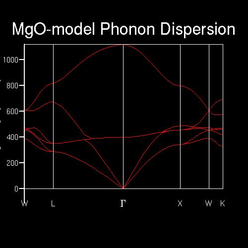 Figure 1. The Phonon Dispersion varies with the frequencies in k-space

Output File: File:MgOdisperC.out
After obtaining the curve, the phonon modes listed in the by the panel can be visualized using Animate Model. The vibration mode 117 (GULP, phonon 4, 399.8 cm-1, 0.000 0.000 0.000) occurred inside the primitive cell due to its k-space point coordinate, and the vibration was shown to be the oxygen atom oscillating within the cell while the 8 magnesium atoms remaining still.
The Phonon Density of States (DOS)
The DOS against Frequency grpahs were camputed using Phonon DOS calculation of GULP.
Different shrinking factors indicated different curve behaviors in the graphs
| Shrinking Factor | 1x1x1 | 2x2x2 | 4x4x4 | 6x6x6 |
|---|---|---|---|---|
| Data Graph |  |
 |
 |

|
| Output Files | File:XwDOS1.out | File:XWDOS2.out | File:XWDOS4.out | File:XWDOS6.out |
| Shrinking Factor | 8x8x8 | 12x12x12 | 20x20x20 | 30x30x30 |
| Data Graph |  |
 |
 |

|
| Output Files | File:XWDOS8.out | File:XWDOS12.out | File:XWDOS20.out | File:XWDOS30.out |
First by comparing the DOS vs Frequency graph of 1x1x1 shrinking factor in Table 2 with the Phonon Dispersion curves in Figure 1, it could be worked out that the DOS for 1x1x1 grid was computed from the k-point of L(1/2 1/2 1/2) which had four intersections where the frequency values were around 290, 350, 680 and 805 cm-1.
Also, the DOS intensity of the frequencies of 290 and 350 cm-1 are approximately twice the DOS intensity of 680 and 805 cm-1 in the DOS graphes. And this could be explained by the double degeneracy of 290 and 350 cm-1.
The frequency values of the four peaks in DOS graph of 1x1x1 grid were the same as the four intersections of the point L.
As shown in the Table 2, as the shrinking factor increases, the number of peaks in the DOS graphs increases and peaks starts to become spread out from 4x4x4.
Until the 8x8x8, the DOS shape shows the obvious increase of peak numbers with density spread out, which means more and more vibrational modes are available.
From 16x16x16, distinct peaks over the frequency range start to emerge and a curve appears instead.
The curve throught the frequency range indicates all frequencies in the range can lead to the corresponding vibrational modes.
The shrinking factors are used to define the size of grid, which indicates that as the size of grid increases, the DOS become spread out through the wavelength range as a curve rather than just peaks present.
The smooth shapes of DOS curve of 30x30x30 and 20x20x20 have little difference, and both of them resemble the shape of 16x16x16 which is a little bit noisy. This means after 16x16x16, there could be another shrinking factor which can give a good approximation of the system.
This optical shrinking factor can be a good point for the calculation of energies and other related properties with a reasonable accuracy.
Computing the Free Energy with The Harmonic Approximation
| Shrinking Factor | Free Energy/ eV | Shrinking Factor | Free Energy/ eV |
|---|---|---|---|
| 1x1x1 | -40.930301 | 12x12x12 | -40.926481 |
| 2x2x2 | -40.926609 | 13x13x13 | -40.926482 |
| 3x3x3 | -40.926432 | 14x14x14 | -40.926482 |
| 4x4x4 | -40.926450 | 15x15x15 | -40.926482 |
| 5x5x5 | -40.926463 | 16x16x16 | -40.926482 |
| 6x6x6 | -40.926471 | 17x17x17 | -40.926482 |
| 7x7x7 | -40.926475 | 18x18x18 | -40.926483 |
| 8x8x8 | -40.926478 | 19x19x19 | -40.926483 |
| 9x9x9 | -40.926479 | 20x20x20 | -40.926483 |
| 10x10x10 | -40.926480 | 30x30x30 | -40.926483 |
| 11x11x11 | -40.926481 | 50x50x50 | -40.926483 |
As shown in Table 3, the free energy values increases as the shrinking factor increases, and the values are convergent to a value which is -40.926483 as shown above.
The energy values of shrinking factors that are greater or equal to 3x3x3 are accurate to 1meV which is 0.001 eV.
The energy values of shrinking factors that are greater or equal to 4x4x4 are accurate to 0.1meV which is 0.0001 eV.
As the value -40.926483 was first obtained in 18x18x18 shrinking factor, so 18x18x18 is the good starting value for the lastter thermal properties' calculations.
Thermal Expansion of MgO
By setting the shrinking factor as 18x18x18, the free energies, lattice constants and the cell volumes were calculated from 0 K to 2800 K in steps of 100 K for 0-1000 K and 200 K for 1000-2800 K.
The calculations were simply carried out using Phonon DOS but with different temperature values.
| Temperature/ K | Free Energy/ eV | Lattice Constant/ Å | Cell Volume/ Å3 |
|---|---|---|---|
| 0 | 0.172485 | 2.986563 | 18.36496 |
| 100 | -40.902420 | 2.986563 | 18.836494 |
| 200 | -40.909377 | 2.987605 | 18.856202 |
| 300 | -40.928124 | 2.989391 | 18.890025 |
| 400 | -40.958594 | 2.991630 | 18.932508 |
| 500 | -40.999435 | 2.994136 | 18.980113 |
| 600 | -41.049315 | 2.996821 | 19.031224 |
| 700 | -41.107119 | 2.999645 | 19.085060 |
| 800 | -41.171891 | 3.002590 | 19.141319 |
| 900 | -41.243017 | 3.005637 | 19.199641 |
| 1000 | -41.319848 | 3.008786 | 19.260045 |
| 1200 | -41.488739 | 3.015392 | 19.387171 |
| 1400 | -41.675513 | 3.022436 | 19.523334 |
| 1600 | -41.877959 | 3.029977 | 19.669831 |
| 1800 | -42.094427 | 3.038113 | 19.828684 |
| 2000 | -42.323671 | 3.046989 | 20.002960 |
| 2200 | -42.564750 | 3.056836 | 20.197505 |
| 2400 | -42.816992 | 3.068052 | 20.420640 |
| 2600 | -43.079960 | 3.081440 | 20.689113 |
| 2800 | -43.353556 | 3.099261 | 21.050132 |
-
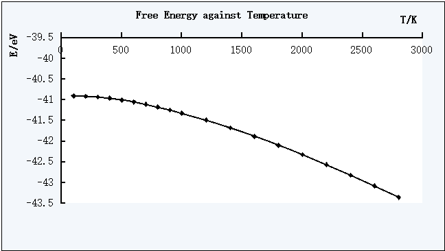 Figure 2. The plot of Free Energy against Temperature

-
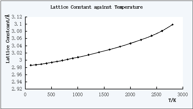 Figure 3. The plot of Lattice Constant against Temperature

-
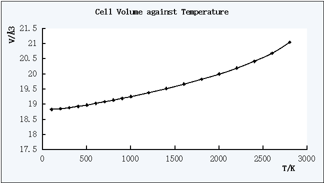 Figure 4. The plot of Cell Volume against Temperature

All of the plots showed smooth curves as Figure 1, Figure 2 and Figure 3 shown above.
The T=0 K data points were not plotted inside the graphs, this is to the zero-point energy values appeared. To obtain more reliable free energy against T graph, the calculations for 0-100 K should be carried out.
The description of the curve lines in the plot can be expressed by each equation if the trend line could be used. In the three plots, the relationships are not completely linear as the observable different increase with each same T interval change. Therefore, a polynomial expression could be better than linear expression for the curves above.
The free energy decreases as the temperature increases, while the lattice constant and the cell volume increases as the temperature increases.
For the Cell Volume against T plot, a trend line can be used to find out the coefficient of thermal expansion as shown below.
-
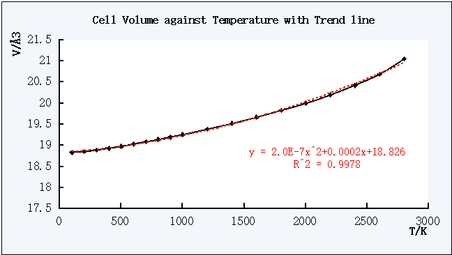 Figure 5. The plot of Cell Volume against Temperature with a trend line

The R2 value 0.9978 which is very close to 1 indicates that this polynomial trend line is a good expression of the relationship between V and T.
To find the thermal expansion coefficient, the equation of this plot is required.
According to the general form of the coefficient of thermal expansion αV =(∂V/∂T)/V with unit of K-1,[3] and the equation obtained in Figure 5 which is y = 2*10-7*x2 + 0.0002*x + 18.826 , therfore, ∂V/∂T = 4.0*10-7*T + 0.0002 which was then substituted back to the general form of the coefficient of thermal expansion to obtain the value for at T.
Therefore, Excel was used to calculate each coefficient value of each V against T data point, and the plot of coefficient of thermal expansion against T was obtained below.
-
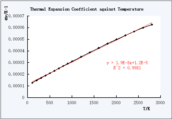 Figure 6. Linear trend line of αV against T
 -
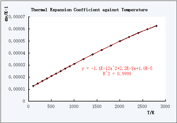 Figure 7. Non-linear trend line of αV against T


The closer the R2 value to 1, the better the expression is.
As shown in the Figure 6 and Figure 7, the polynomial non-linear equation was better one to describe the relationship between the coefficient of thermal expansion and T.
The theoretical/experimental value of the Linear Coefficient of Thermal Expansion is (12.6 +/- 0.5)*10-6 K-1 in the Temperature range of 1000-2000 celsius degrees.[4] And 1000-2000 celsius degrees is the same as 1275-2275 K.
The coefficient values in the Figure 6 and Figure 7 was in the range of 12.7412*10-6-62.7074*10-6 K-1 with the T range of 100-2800 K.
The 1275-2275 K is within the range of 100-2800 K and the coefficient range (12.6 +/- 0.5)*10-6 K-1 is not within 12.7412*10-6-62.707*10-6 K-1, which indicates some extent of the accuracy from the calculations.
In the quasi-harmonic approximation which was used in the calculations above, all of the phonon modes were assumed to be harmonic and resemble the 1D harmonic potential.
Molecular Dynamics Calculations
In this calculation method, the parameter of dT and size were considered.[2] Therefore, a model with 32 units of MgO was used instead, which allowed the flexibility to be performed.
| Temperature/ K | Average Volume/ Å3 |
|---|---|
| 100 | 599.552364 |
| 200 | 600.513626 |
| 300 | 602.899441 |
| 400 | 603.241540 |
| 500 | 605.731599 |
| 600 | 607.831884 |
| 700 | 609.326722 |
| 800 | 612.059646 |
| 900 | 613.477026 |
| 1000 | 615.053673 |
| 1200 | 620.019685 |
| 1400 | 622.667240 |
| 1600 | 626.171861 |
| 1800 | 630.981406 |
| 2000 | 632.416616 |
| 2200 | 637.036302 |
| 2400 | 642.621784 |
| 2600 | 648.409448 |
| 2800 | 655.021355 |
The cell volume per formula unit for the data in Table 4 can be calculated using Cell Volume(per formula) = Average Volume/32.
The calculations for the Coefficient of Thermal Expansion wsa the same as the one used in the quasi-harmonic approximation method which used αV =(∂V/∂T)/V.
-
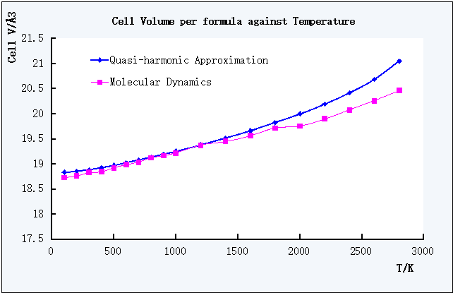 Figure 8. Plot of Cell Volume per formula against T of QHA and MD

-
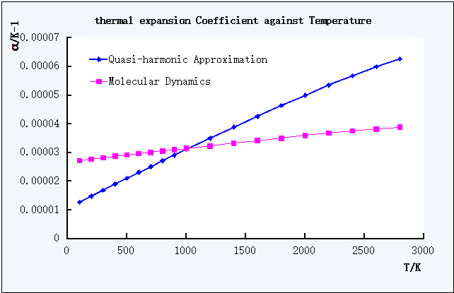 Figure 9. Plot of Coefficient of Thermal Expansion against T of QHA and MD

The coefficient values obtained from Molecular Dynamics calculations in the Figure 9 was in the range of 26.9695*10-6-31.6765*10-6 K-1 with the T range of 100-2800 K.
The theoretical/experimental value of the Linear Coefficient of Thermal Expansion is (12.6 +/- 0.5)*10-6 K-1 in the Temperature range of 1275-2275 K.[4]
Although the MD curve in Figure 9 showed a good linearity, the experimental values range was not within the values range from the calculation using Molecular Dynamics, this might indicated the MD calculation was not suitable for the calculation of this temperature range.
To be more accurate, the specific theoretical Coefficient of thermal expansion at each temperature point are required and the theoretical/experimental coefficient values of MgO at higher temperature are necessary for the comparisons.
In the Figure 8, the curve plotted for Molecular Dynamics was more fluctuated than QHA, the polynomical equation was given as y = 5.3*10-8*x2 + 0.005*x +18.691, therefore ∂V/∂T = 1.06*10-7*T + 0.0005 and the calculations of coefficients were using EXCEL.
In Figure 9, both curves resembled linear trend, which indicated the linear thermal expansion of MgO under both calculation methods. However, it could be observed that the increase of the coefficient with increasing T of MD was slower than QHA according to the smaller gradient of the curve of MD.
Conclusion
Both Molecular Dynamics and QHA calculation methods indicated a good linearity in the Coefficient of thermal expansion against temperature graphs.
Molecular Dynamics calculation results showed much a greater deviation in the Coefficient values than QHA, which might be due to the temperature range chosen in the calculations were not high enough for MD acting as an accurate method.
Instead, the extent of accuracy of QHA calculation method indicated that it might be a better method whthin the temperature range used in this computaional exercise. But if higher temperature was used, QHA could then be inaccurate, because the limitation which indicated that the potential-distance potential model became more and more poor with T increasing become a great factor.
Therefore, at high T, Molecular Dynamics could be a better method.
The extent of inaccuracy of both methods could come from the limitations of each methods like the assumptions and the temperature range.
Also, the experimental values were based on large system while the two computational methods were based on single cell or a few more cells. If larger systems can be calculated using the two methods and a much greater range could be used, the accuracy and deviations of data might be more obvious.
References
- ↑ WIKIPEDIA, Phonon, Available from: https://en.wikipedia.org/wiki/Phonon [Accessed: 24th January 2016]
- ↑ 2.0 2.1 3rd Year MgO Computational Script, Molecular Dynamics, Available from: http://www.ch.ic.ac.uk/harrison/Teaching/Thermal_Expansion/md.html [Accessed: 25th January 2016]
- ↑ WIKIPEDIA, Thermal Expansion, Available from: https://en.wikipedia.org/wiki/Thermal_expansion#General_volumetric_thermal_expansion_coefficient [Accessed: 25th January 2016]
- ↑ 4.0 4.1 CHARLES J. ENGBERG, ERNEST H. ZEHMS, Thermal Expansion of AI,O,, BeO, MgO, B,C, Sic, and Tic Above 1000°C , Journal of the American Ceramic Society., 1959, 42(6), pp 300-305. DOI: 10.1111/j.1151-2916.1959.tb12958.x