Rep:Liquids GE715

The sections of your report are a little bare and would have been nice to see you elaborate a little more and maybe suggest some additional simulations you could undertake. Also would have been good to go through your tasks. Mark: 57/100

Abstract

In this experiment properties of liquids were modelled using molecular dynamics experiments. The effect of the temperature on the density as well as the effect of temperature on the heat capacity, and the radial distribution functions were explored.

Introduction

Not much of an introduction - this should serve to overview the work, target your audience (provide an interesting application for your work; why is it a hot topic?) and give a literature overview/review.

Molecular dynamics is a modern would say it's more classical! (pun intended) computational technique concerned with calculating properties of substances by modelling them and their behaviour on atomic level with powerful computers.

Lennard Jones potential equals $ϕ (r) = 4 ϵ (\frac{σ^{12}}{r^{12}} - \frac{σ^{6}}{r^{6}})$ . Potential energy is zero at the point when $r = σ$ , thus $r_{0} = σ$ .

Force is simply the derivative of the potential, thus $F = 4 ϵ (- 12 \frac{σ^{12}}{r^{13}} + 6 \frac{σ^{6}}{r^{7}})$ . At $r = σ$ this equals $F = - \frac{24 ϵ}{σ}$ . Well depth is $ϕ (r_{e q}) = - ϵ$ , where $r_{e q} = σ \sqrt[6]{2}$ .

The following integrals are equal to: $\int_{2 σ}^{\infty} ϕ (r) d r = - 0.0248$ , $\int_{2.5 σ}^{\infty} ϕ (r) d r = - 0.00818$ , and $\int_{3 σ}^{\infty} ϕ (r) d r = - 0.00329$ .

Introductory tasks

Water

There are roughly $3.3 * 1 0^{22}$ molecules in 1 mL of water. However, 10000 atoms of water take up about $3 * 1 0^{- 19} m L$ or $300 n m^{3}$ . This is a good illustration of how different atomic scale is from the scale on which the properties of substances tend to be observed.

Atoms

Atom at position $(0.5, 0.5, 0.5)$ moved for $(0.7, 0.6, 0.2)$ would be found at $(0.2, 0.1, 0.7)$ , since it would be copied in both x and y direction (assuming x,y,z).

Reduced units

Lennard-Jones parameters for argon were given, the macroscopic properties are calculated here.

$L J_{c u t - o f f} = 1.088 n m$

$T = 180 K$

$r = 0.382 n m$

$E = 1 \frac{k J}{m o l}$

Aims and Objectives

This is quite brief - you're very welcome to use bullet points in your aims and objectives. Especially for your thesis!

The aim of this experiment was to explore the modern use of molecular dynamics for simulating simple liquids.

The objectives were to look at how timesteps used in experiment affect the quality of the results, how temperature affects density and find radial distribution functions and their integrals for different phases of matter.

Methods

A computational methods section should start by describing the model used. Then all the tools and techniques you used. Again this is too brief.

The calculations were performed on a high performance computer using LAMMPS software package, while the calculations of radial distribution functions were done using VMD (delta r=0.05).

Equilibration

If two atoms were generated very close together that would mean the force between them would be enormous you're right here but enormous is hardly the most scientific of language!, which would have a potential to heavily disturb the simulation (very high potential energy would increase the temperature).

Commands =

mass 1 1.0 signifies that the mass of the first kind of particles (1) is 1.0.

pair_style lj/cut 3.0 tells us where the interactions are cut off, as seen in the integral above, $3.0 σ$ is a very good cut-off, since there is no significant perturbation.

The algorithm used for the calculations is velocity-Verlet, because the classical one does not use velocities.

Simulations

In the gallery below graphs are shown. It can be seen that as timesteps are increasing, the quality of results is decreasing. Timpestep of 0.015 s is wholy inappropriate, but I have chosen to run the experiments at the timestep of 0.0025 s. why did you choose this timestep? Results would probably also be almost as good using 0.01 s. We can see this by the fact that equilibrium is reached very quickly, for the first for timesteps in the space of 0.1 s -0.3 s. The highest timestep will mimic the reality better, but it might be too demanding computationally.

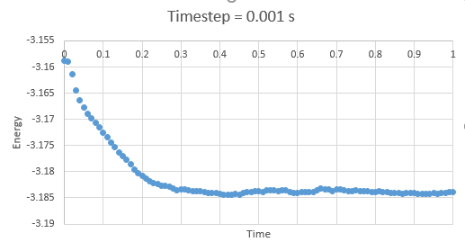Figure 1: Energy at timestep 0.001 s
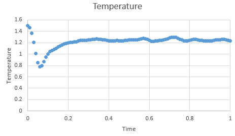Figure 2: Temperature at timestep 0.001 s
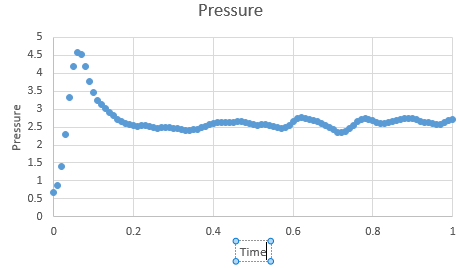Figure 3: Pressure at timestep 0.001 s
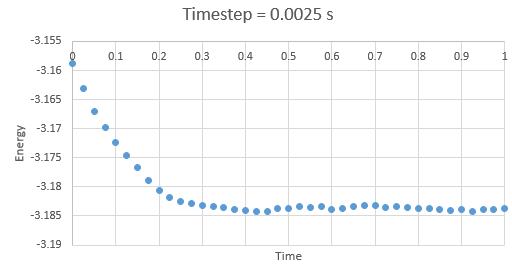Figure 4: Energy at timestep 0.0025 s
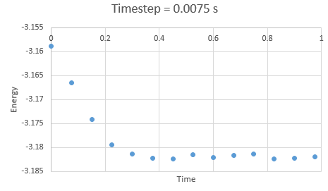Figure 5: Energy at timestep 0.0075 s
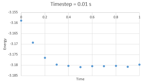Figure 6: Energy at timestep 0.01 s
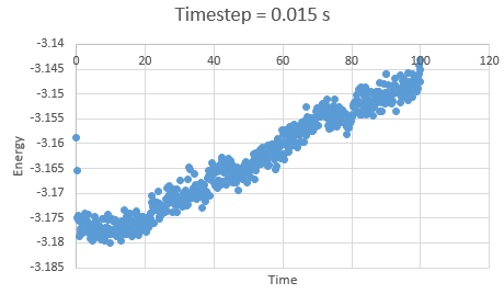Figure 7: Energy at timestep 0.015 s

Specific conditions

Should have tried to plot these on the same graph to see how the simulation data tends towards ideality at high temperatures

The next task was to run simulations varying temperatures at constant pressure. This shows the dependence of density on temperature at a constant pressure. Considering the ideal gas law the density will be inversely proportional with temperature.

If we run simulations under different conditions, we get the results shown in the gallery below. Bear in mind that some errors are almost negligible.

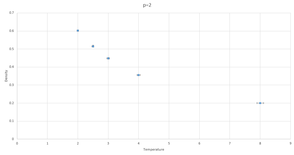Figure 8: Density vs temperature at p=2
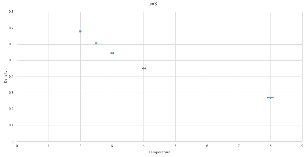Figure 9: Density vs temperature at p=3
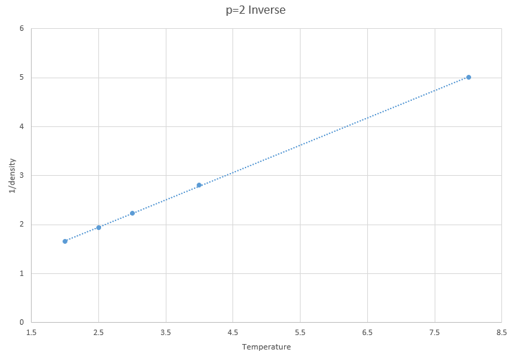Figure 10: Inverse of density vs temperature at p=2
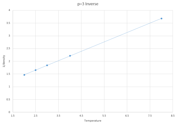Figure 11: Inverse of density vs temperature at p=3

The inverses are of densities are shown to prove that this simulation obeys the proportionality proposed ideal gas law, where the density and temperature are inversely proportional.

Heat capacity calculation

Heat capacity at constant volume may be calculated using equation $C_{V} = N^{2} \frac{⟨ E^{2} ⟩ - {⟨ E ⟩}^{2}}{k_{B} T^{2}}$ , which LAMMPS software enables us to do. This was done at two different densities (0.2 and 0.8) and is shown in the gallery below.

Figure 12: Heat capacity per volume vs temperature at d=0.2
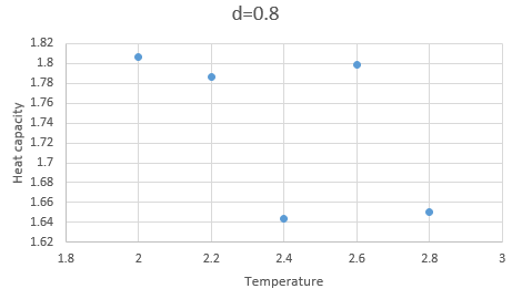Figure 13: Heat capacity per volume vs temperature at d=0.8

Any trends in heat capacity over a range of temperatures at a fixed volume is not entirely clear even though we would normally expect a gradual decrease in heat capacity with higher temperatures. should we expect a gradual decrease? Constant number of particles, constant internal energym Cv = dU/dT therefore Cv should be constant...

An example of the code used to calculate this is shown below (d=0.2, T=2.0). Heat capacity was finally divided by a volume.

### DEFINE SIMULATION BOX GEOMETRY ###
variable dens equal 0.2
lattice sc ${dens}
region box block 0 15 0 15 0 15
create_box 1 box
create_atoms 1 box

### DEFINE PHYSICAL PROPERTIES OF ATOMS ###
mass 1 1.0
pair_style lj/cut/opt 3.0
pair_coeff 1 1 1.0 1.0
neighbor 2.0 bin

### SPECIFY THE REQUIRED THERMODYNAMIC STATE ###
variable T equal 2.0
variable timestep equal 0.0025

### ASSIGN ATOMIC VELOCITIES ###
velocity all create ${T} 12345 dist gaussian rot yes mom yes

### SPECIFY ENSEMBLE ###
timestep ${timestep}
fix nve all nve

### THERMODYNAMIC OUTPUT CONTROL ###
thermo_style custom time etotal temp press
thermo 10

### RECORD TRAJECTORY ###
dump traj all custom 1000 output-1 id x y z

### SPECIFY TIMESTEP ###

### RUN SIMULATION TO MELT CRYSTAL ###
run 10000
unfix nve

### BRING SYSTEM TO REQUIRED STATE ###
variable tdamp equal ${timestep}*100
fix nvt all nvt temp ${T} ${T} ${tdamp}
run 100000
reset_timestep 0

### MEASURE SYSTEM STATE ###
thermo_style custom atoms etotal temp vol
variable N2 equal atoms*atoms
variable E equal etotal
variable E2 equal etotal*etotal
variable temp equal temp
variable temp2 equal temp*temp
variable vol equal vol
fix aves all ave/time 100 1000 100000 v_E v_E2 v_temp2
run 100000

variable heatcapac equal N2*(f_aves[2]-f_aves[1]*f_aves[1])/(f_aves[3])

print "Averages"
print "--------"
print "Heat Capacity: ${heatcapac}"
print "Volume: ${vol}"

Radial distribution functions

The radial distribution functions from the calculations are given in the gallery below.

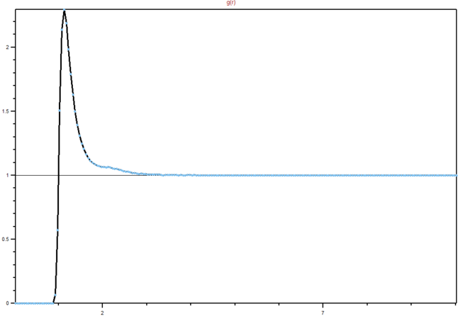Figure 14: RDF for a gas
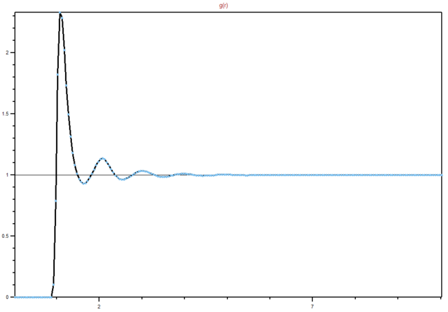Figure 15: RDF for a liquid
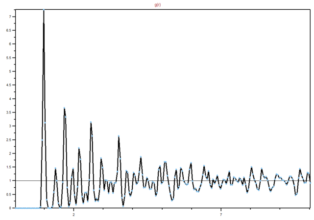Figure 16: RDF for a solid
Figure 17: Integral of RDF for a gas
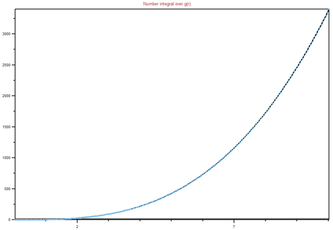Figure 18: Integral of RDF for a liquid
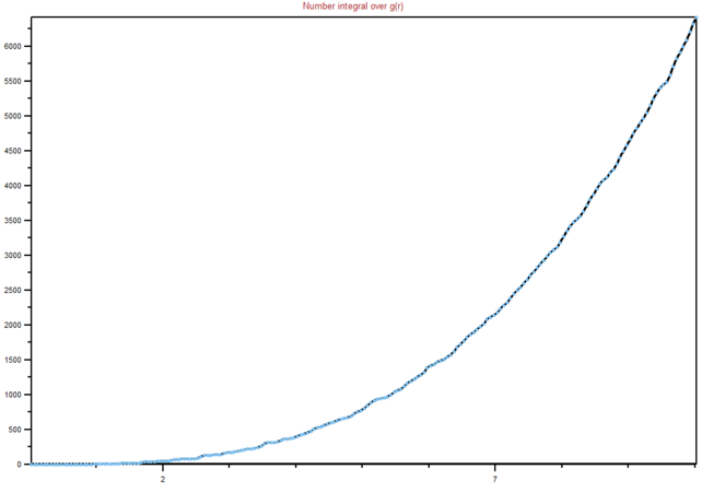Figure 19: Integral of RDF for a solid

We can see from the graphs the differences between different phases and their order. It is clear that in a solid lattice structure is fairly rigid (peaks are the neighbouring atoms), liquid is slightly less ordered, while gas has almost. no real order at all. Lattice spacing in a solid is $σ$ , while the first peak represents the nearest neighbouring atoms, while the next two represent the atom that are not nearest neighbours, but are less than two atoms away in a straight line from the central atom. The interactions are dropping of with distance, as expected in Lennard-Jones model. You're right that the rdf shows the inherent order for a system of particles. For a liquid, the peaks are smooth because of dynamic averaging. Gas has no long-range order, whilst a liquid has some shells of correlation.

Conclusion

Although these are take home messages would be good to connect this back to your introduction. Also giving your conclusion a little more "meat" wouldn't go amiss! It has been determined that appropriate timestep for dynamics calculations is 0.0025 s.

Simulations were performed to determine that temperature and density of a liquid are inversely proportional.

Another finding was that heat capacity does not necessarily have a clear strong dependence on temperature at constant volume.

It was also found that radial distribution function depends heavily on the phase of matter, with order being clearly seen in solid lattice.