Rep:LiquidSimulationkbg15

Some of the tasks have not been included as an appendix in the Q&A style requested, but instead morphed into a report. I combed through your report and picked out the tasks, awarding you the marks. However, it is difficult to write a good scientific report by lumping together a bunch of disparate tasks. This has indeed negatively effected the quality of your report, which should be concise, clearly motivated and progress in a logical manner. Some of the tasks are missing altogether. Your report would have benefited from some proof reading / grammar checks, and a more formal/scientific writing style. From your aims and objectives section, it is evident that you were not trying to perform a scientific investigation, and perhaps misunderstood the task. Plots do not require both a caption and title. On the whole, you have demonstrated a grasp of the basic principles of molecular dynamics. You have an impressive number of citations, and this is evidence of effort/further reading on your part. It's also good that you did the extension material.

Abstract

The research achieved the usage of computational simulation to estimate thermodynamic properties of real life systems, such as the heat capacity, diffusion coefficient, internal energy, total energy and etc. These properties explain the nature of states (solid, liquid and gas), and instil the law of thermodynamics. The simulation also reinforce the deviation of behaviours of real gas from the ideal gas. For example, the decrease of pressure and increase of temperature of a system are good approaches to mimic ideal gas system. Lennard-Jones interaction was used as a primary basis of the simulation to provide first order approximations of the reality of system. A lot of thermodynamic equations were used to explain the simulation results, such as the Einstein relation in Brownian motion, Stokes-Einstein equation, velocity autocorrelation coefficient, and the ideal gas laws, thus further reinforce the applications of these equations both in the simulation and in real life. An abstract is meant to briefly summarise your methodology and results, with a brief motivation. This has not really been achieved - you make a lot of general statements, but fail to impart specifically what you have done. Grammar could also be improved.

Introduction

Computer simulation has become a powerful and useful tool to estimate and solve complicated real problems in life. From building a bridge to designing a stable colloidal suspension, computer simulation is the best estimate before actual trial. Thousands and millions of combinations could have been tried in a computer simulation to screen worthless attempts, and save up cost of money and time in random trials. Moreover, protein folding, DNA coiling, uncoiling and supercoiling could be simulated to allow scientists to understand processes such as translation and transcription, enzymatic activities and antibodies mechanisms. These processes could not be observed under a microscope, but by understanding the molecular forces and the structure of the molecules, models could be built to replicate what the nature does in computer simulation. On the whole this is true, but could be more succinctly put. Also, you are not writing a review on the usefulness of computer simulations in science. The introduction of a scientific paper should provide a concise motivation, review of the underlying theory, and any other salient information.

Different thermodynamic parameters have been estimated using computational simulation of Lennard-Jones fluid. These values were compared with the experimental values to convey experiments out from the lab, into computers. Scientists were trying to use their understanding from the physical phenomena and equations to replicate and simulate a model that represents the reality. This method opened a door to scientists to obtain "experimental" values from computational analysis rather than a lab analysis. Again you make some very general statements. What thermodynamic parameters? You should provide relevant background theory.

Numerical algorithms are useful to solve complicated mathematical equations in computer. From a complicated Schrodinger's equation to a simple harmonic oscillator could be solved using numerical methods. One of those algorithms is the Verlet algorithm which solves the position and velocity using some second order approximations. These powerful algorithms help mankind solve complicated mathematical equations as long as the conditions are reasonable giving relatively small errors. Not a very necessary paragraph.

Aims and Objectives

1. To understand the computational algorithms in solving complex differential equations.
2. To simulate particles with preset interaction type in a system, and obtain results from it.
3. To use simulation results in estimating thermodynamic quantities.
4. To compare and contrast the properties of real gas from simulation and ideal gas.
5. To differentiate the states of matter from the diffusion coefficients which were calculated from simulation.
6. To relate and apply thermodynamic equations in solving real life problems.
7. To understand basic LAMMPS input coding for computational simulation.

Methods

Verlet algorithm to estimate 1-D simple harmonic oscillation

The analytical displacement of the displacement was set as a cosine function. The error was calculated from the absolute difference between the analytical displacement and the displacement obtained from the algorithm. The total energy of the system was the sum of the kinetic energy $\frac{1}{2}m{v}^2$ and the potential energy $\frac{1}{2}k{x}^2$, with both x and v parameters estimated from the algorithm. The peaks of the absolute error were linear fitted using Excel while the percentage error for each time step used were fitted to a quadratic equation using Excel. The percentage error was calculated using maxima-minima/maxima.

Simulation box and parameters

For simulations of liquid and gas, simple cubic lattice structure was used as the initial system, whereas face-centred cubic structure was used in solid simulations. The densities of the liquid simulation used were 0.2 and 0.8 whereas 1.2 for solid simulation and 0.01 for gas simulaiton. Wide range of temperatures were used in different simulations. If not specified, the timestep of the simulations was set to 0.025. This timestep was chosen to give reasonable results and short actual simulation time. 1 atom type (Type 1 atom) with mass 1.0 was used. The pair interactions between particles were the Lennard-Jones potential with a cutoff at $r^{*}=3$. The pair coefficient was set as 1.0 for all the simulations. Graphs were plotted in both Excel and Python, whereas curve fitting was done by polyfit in Python and trend line in Excel. Trapezium rule and running integrals were compiled using Python numpy.trapz function.

I would be able to reproduce your results given the information you have provided - good. However, you do not have to, and should not, credit analysis tools such as excel and python (especially an individual numpy function such as numpy.trapz). This is superfluous information as the analysis could be carried out using many other software packages.

Results and Discussion

Isobaric-isothermal (NpT) ensemble

From equipartition theorem, the total kinetic energy of a 3 dimension system is described as equation below.

$\frac{1}{2}\sum _i{m}_i{v}_i^2=\frac{3}{2}N{k}_{B}T$

However, due to the nature of the simulation, the temperature will fluctuates, and hence we modified the equation slightly with $\mathfrak{𝔗}$ as our target temperature and $\gamma$ as a correction.

$\frac{1}{2}\sum _i{m}_i{\left(\gamma v_i\right)}^2=\frac{3}{2}N{k}_B\mathfrak{𝔗}$

The two equations were used to solve $\gamma$, giving rise to the equation below.

$\gamma =\sqrt{\frac{\mathfrak{𝔗}}{T}}$

The following LAMMPS input

fix aves all ave/time 100 1000 100000 v_dens v_temp v_press v_dens2 v_temp2 v_press2
run 100000 

specify the averaging method of the variables (dens, temp, press, dens2, temp2 and press2). The three numbers 100, 1000 and 100 000 represents the value taken in every interval, number of values used in averaging, and the final averaged quantities generated on timesteps respectively. In layman term, the above input is a systematic sampling method which select values in every 100 data for example, the 100th data, 200th data, 300th data up to the 100 000th data, giving rise to 1000 measurements used to generate the average, and the total average is generated on the 100000th data. The following input line giving the number of steps in the simulation, with timestep of 0.075, a total time of 7500 (100 000*0.075) will be generated. Tick. This explanation was required for one of the tasks, and should be appended to your wiki page. However, should it really go in a report? Scientific papers do not explain the input files they have used. Also, scientific papers are (for better or for worse) aimed at scientists, and using extra words to elaborate in layman's terms is unnecessary.

For ideal gas, the density changes with temperature according to the equation below. The simulation situations at different pressures were compared with the ideal gas situations.

$\rho =\frac{PM}{RT}$

where $\rho$ is the density, P is the pressure, M is the molar mass, R is the gas constant and T is the temperature.

Figure 8: Graphs of density vs temperature with simulation and ideal situation at different values of pressure, p Error in density is too small to be observable in the errorbar.

Figure 9: Graphs of density vs temperature with simulation situation and ideal gas situation at pressure, p = 5 for a larger temperature range.

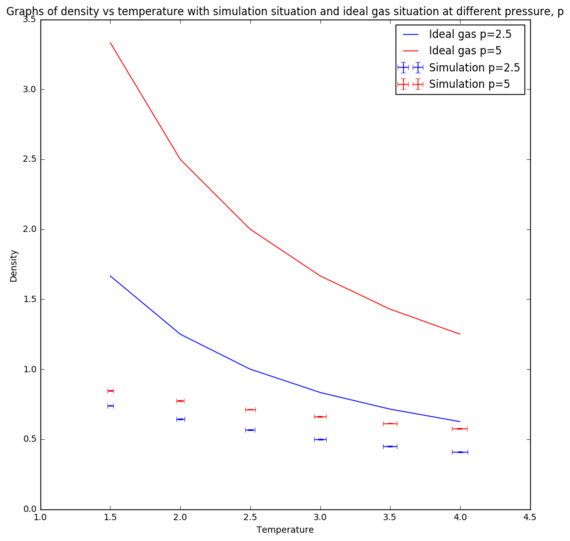
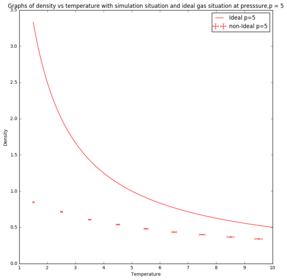
From the graphs in Figure 8 and Figure 9, the simulated density is lower than the ideal gas density. However, at high temperatures, both graphs are converging to same density. This trend could be explained by the interaction between particles in the simulation. Ideal gas ignores all the interactions between particles and assuming particles' volume is neglected. These assumptions were not included in the simulation, hence giving rise to repulsion between particles. Therefore, the inter-particle spacing gets larger, giving rise to a lower simulated density. However, the interaction becomes more negligible at higher temperatures, causing the particles in the simulation behaves more ideally, which hence explains the convergence of the two lines at high temperatures. The discrepancy between the densities of the simulated density and the ideal gas density is larger at high pressure because at higher pressure, the repulsion between the particles are more significant than the repulsion at lower pressure. Therefore, at high temperature and low pressure, particles behave like ideal gas. Tick.

Microcanonical (NVE) ensemble and the specific heat capacity

Figure 10: Graphs of heat capacity / volume, C$_V$/V vs temperature at different densities.

For ideal gas, the internal energy, U is the sum of the kinetic energy and potential energy between all particles. Due to the fact that the potential energy is zero in ideal gas, the average kinetic energy follows the equipartition principle, giving rise to the equation below.

$U=\frac{3}{2}NkT$

Where N is the number of particles, k is the Boltzmann constant, and T is the temperature.

Since the thermodynamic representation of the specific heat capacity at constant volume is the partial derivative of the internal energy respect to temperature at constant volume, the heat capacity of ideal gas hence follows the equation below. For reduced form of this quantity, the Boltzmann constant is equal to 1 and the number of particles and volume are constant in the ensemble, the specific heat capacity of ideal gas is hence a constant regardless of the temperature. Tick.

$C_V={\left(\frac{\partial U}{\partial T}\right)}_V=\frac{3}{2}Nk$

From the section above, we noticed that in the simulation, particles deviates from the ideal behaviour. Therefore, in Figure 10, the quantity $C_V/V$ decreases with temperature.

Due to similar argument from the section above, simulated particles have interaction between one another and take up space, they repel each other, and cause the larger heat capacity compared to the ideal gas. The larger heat capacity explains more energy is needed to raise the temperature of the system as energy is used to break interactions between particles, allowing them to access higher translational states. Hence, the larger the heat capacity, the more deviated from ideal behaviour the system is. As particles behave ideally and high temperature and low pressure, increasing the temperature decreases the heat capacity; whereas increasing the density increases the pressure, which therefore increases the heat capacity.

Radial distribution function of different states

Figure 11: Radial distribution funciton, g(r) for different states.

The radial distribution function, g(r) describes the density or in other word probability of finding a particle at a radial thin shell away from the centre of a particle with radius, r. the initial g(r) for all three states before r*=1 is zero, because no particles could be possibly found in that region. The g(r) of gas increases rapidly after r*=1 and reaches it's maximum before decreases and plateau at 1. This behaviour could be explained as gas particles have a single coordination sphere at the radius which gives the peak of g(r). This is the distance which the Van der Waals forces are the strongest, and it quickly decays to bulk density of gas, giving rise to the plateau of g(r) at 1 for larger particle separation. For g(r) of liquid, few peaks could be seen before the plateau, which signifies the few coordination spheres before the bulk density of liquid. The interaction strength between particles in liquid is larger, giving rise to first, second and even third coordination spheres. The peaks get smaller due to the depleted probability of finding particles outside the first coordination sphere which is caused by repulsion by the first coordination sphere.

Figure 12: The lattice packing in face-centred cubic unit cell.

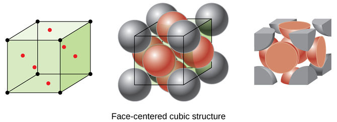
However, in face-centred cubic solid, the infinite regular packing of the unit cells give rise to constant intervals of the peaks in the g(r). The peaks occur at $1\sigma$,$\sqrt{2}\sigma$ and $\sqrt{3}\sigma$represents the lattice packing of the solid. By imagine the black dot on the upper right back corner of the cubic unit cell in Figure 12, the three red particles closest to the black dot give rise to the first coordination sphere, which the distance is $\frac{1}{\sqrt{2}}a$ where $a$is the lattice spacing. A total of 12 red dots surround the black dot in repeating unit cells. The second coordination sphere will be the closest three black particles, which the distance is $a$from the black dot. A total of 6 black dots surround the black dot in repeating unit cells. The third coordination sphere will be the other three red dots, which the distance is $\sqrt{\frac{3}{2}}a$ away from the black dot, with a total of 12 red dots surround the black dot in repeating unit cells. By knowing $\sigma =\frac{1}{\sqrt{2}}a$, the distance of the coordination spheres from a particle will be $1\sigma$,$\sqrt{2}\sigma$ and $\sqrt{3}\sigma$ as shown. The lattice spacing, hence is equal to the distance of the second coordination sphere from a particle with $r^{*}=\sqrt{2}\approx 1.414$

Figure 13: Graphs of $\int g(r)dr$ against $r$ for different states

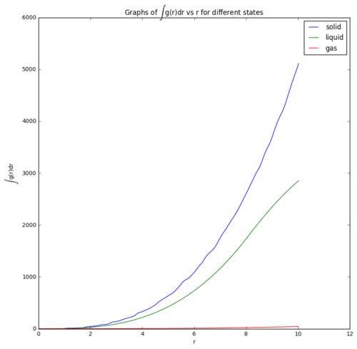
Moreover, the coordination number could be predicted using the integration of g(r) in spherical coordinates, which gives rise to the probability of finding particles in that distance away from a particle, then multiply by the number density to get the coordination number, n(r) as shown in equation below. $n(r)=\rho \underset{0}{\overset{r^{\prime }}{\int }}g(r)4\pi r^{2}dr$

However, the number of particles, N is directly proportional to the integral of g(r) as shown in equation below. Therefore, the graphs in Figure 13 shows that the curvature of graph is largest in solid and smallest in gas. This is due to the large density of particles in solid, which gives rise to large number of particles in the sphere with radius r. Relatively smaller density of liquid has smaller curvature in the graph whereas the least dense gas state has a smallest curvature of the curve.

$N\propto \int g(r)dr$

Diffusion coefficient and Mean Square Displacement (MSD)

In the Einstein's relation for Brownian motion, the mean square displacement, $<x^2>$ is related to the time in equation below.

$<x^2>=2dDt$

Where d is the dimension, which equals to 3 in 3-d space and D is the diffusion coefficient.

The diffusion coefficient, D is related to the Stokes-Einstein equation as follow,

$D=\frac{k_{B}T}{6\pi \eta r}=\frac{1}{6}\frac{\partial ⟨r^2\left(t\right)⟩}{\partial t}$

Figure 14: Graphs of mean square displacement vs time for solid, liquid and gas.

Table 1: Estimated diffusion coefficient from the graphs in Figure 14 using Einstein relation

State	Diffusion coefficient from 1 million particles	Diffusion coefficient from thousands of particles
Solid	0.0000003352	0.000002004
Liquid	0.006434	0.006569
Gas	0.2316	0.5714

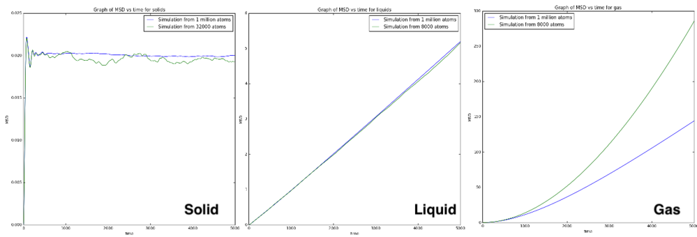
From Figure 14, the graphs of mean square displacement vs time of solid liquid and gas were plotted. The mean square displacement plateau at a value in solid. This value arises from the vibration of particles in the lattice. Due to the high activation energy to remove an atom from solid lattice, the relaxation time is very large, giving rise to a very small diffusion coefficient in solid. Therefore, from the equation above, the gradient of the graph is very close to zero. In liquid, the graph is linear, giving rise to a constant gradient and a constant value of diffusion coefficient. The temperature used for both of the graphs in liquid was the same, giving rise to the same diffusion coefficient. For gas, the particle separation is too large, giving rise to Ballistic motion described from the equation below. The kinematic motion gives rise to a quadratic relation between MSD and time, which in other word means there is negligible activation energy to move particle from one place to another. The difference in the curves generated from different number of particles is because of the different temperature used in the simulation. The general trend of the diffusion coefficients is logical with solid has the smallest diffusion coefficient and gas has the largest diffusion coefficient. For the unit of the diffusion coefficient, since the distance is recorded in reduced unit, the mean square displacement is in reduce unit as well which is unit-less. Therefore, the diffusion coefficient has the unit of inverse time.

$<x^2>=\frac{3kT}{m}{t}^2$

=== Extension: Velocity Autocorrelation Function, VACF === You should use our task title "extension" in a scientific report.

Figure 15: Graphs of VACF vs time for solid, liquid and simple harmonic oscillator, SHM.

The normalised velocity autocorrelation function is described as the equation below.

$C\left(\tau \right)=\frac{\underset{-\mathrm{\infty }}{\overset{\mathrm{\infty }}{\int }}v\left(t\right)v(t+\tau )\mathrm{d}t}{\underset{-\mathrm{\infty }}{\overset{\mathrm{\infty }}{\int }}{v}^2\left(t\right)\mathrm{d}t}$

It can be used to estimate the diffusion coefficient using the equation below.

$D=\frac{1}{3}\underset{0}{\overset{\mathrm{\infty }}{\int }}\mathrm{d}\tau ⟨\mathbf{v}\left(0\right)\cdot \mathbf{v}\left(\tau \right)⟩$

The velocity of a simple harmonic oscillator is described as the equation below. This equation is obtained by assuming the displacement as a cosine function of time.

$v=-sin(\omega t)$

Substituting the velocity into the VACF, cosine function is obtained. Correct result.

$C\left(\tau \right)=\frac{\underset{-\mathrm{\infty }}{\overset{\mathrm{\infty }}{\int }}-sin(\omega t)\times -sin(\omega (t+\tau ))\mathrm{d}t}{\underset{-\mathrm{\infty }}{\overset{\mathrm{\infty }}{\int }}(-sin(\omega t){)}^2\left(t\right)\mathrm{d}t}=cos(\omega \tau )$

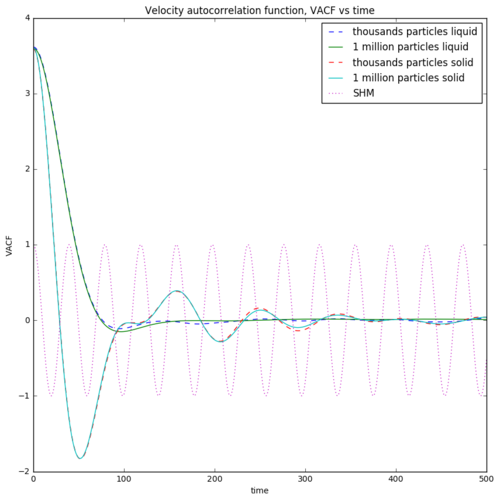
The graphs of the VACF vs time for solid, liquid and simple harmonic oscillator are plotted in Figure 15. For solid, due to the high activation energy to remove a particle from the coordination spheres, the particles can only vibrate. Particles moving at high initial velocity to a direction moves backward in an opposite direction with a negative sign. Therefore, the particles show no net movement throughout the simulation. For liquid, the particles have smaller activation energy to move away from the coordination spheres. Liquid hence exhibit flow properties. The high initial velocity decreases to zero but particles never move backward, causing a net movement of particles. This give rise to the diffusion coefficient. Due to the fact that the integral of the VACF in solid will causes the positive phase cancelling out the negative phase, the diffusion coefficient which is directly proportional to the integral is very close to zero. This statement further proves the inability of particle flow in solid. For liquid, the integral gives a net positive value, resulting a diffusion coefficient which explains the flow property of liquid. The diffusion coefficient estimated using VACF is tabulated below. Due to the nature of the harmonic oscillator, the VACF is a regular cosine function. The large velocity towards one direction will cancelled out with another velocity pointing towards the opposite direction. Therefore, particles under simple harmonic motion can never disappear from the system.

Table 2: Estimated diffusion coefficient from the integral of VACF

State	Diffusion coefficient from 1 million particles	Diffusion coefficient from thousands of particles
Solid	0.02276	0.02276
Liquid	45.05	39.16

Figure 16: Graphs of running integral of VACF against time

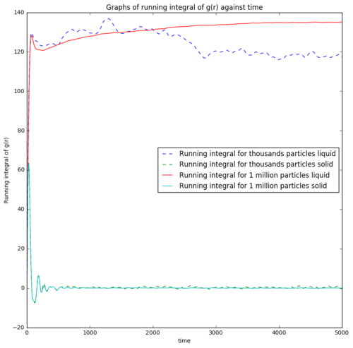
The areas under the curves used in estimating the diffusion coefficient were calculated using the trapezium rule. The running integral of the VACF against time is also plotted in Figure 16. The integral of VACF for solid initially is high, but quickly reduces and plateau at zero showing the cancelling effect of the opposite direction velocities against the initial velocities. However, the running integral for liquid starts at the same point but increases and plateau, showing flow properties with diffusion coefficient. Error from the estimate of diffusion coefficient from integral of VACF could be arising from the trapezium rule. A larger possible error is due to the most contributing part to the integral of VACF comes from the earlier part of the simulation which the system might not reach equilibrium yet. This error which came from the nature of the integration algorithm contributes largely to the contradiction of the estimated diffusion coefficient from integral VACF and ones from mean square displacement which uses later part of the simulation.

Conclusion

Simple LAMMPS input script was comprehended and was used to simulate systems which reflect the reality. The Verlet algorithm was used to estimate the behaviour of the systems. Simulation results such as the total energy, temperature, density, mean square displacement (MSD) and velocity autocorrelation function (VACF) were used to estimate the heat capacity, duration for the system to reach equilibrium, the diffusion coefficient, the lattice spacing of the matter, coordination spheres and the coordination numbers. Real gas behaved more like ideal gas by increasing the temperature and decreasing the pressure of the system. The properties of the states of matter were reflected from the simulation results. For example, small integral VACF or constant plateau MSD indicates a solid system. Thermodynamic equations were satisfied from the simulation results, thus estimated parameters such as the diffusion coefficient, and explained the behaviour of MSD over time and the deviation of results from the ideal gas equations.

Appendix I - Theory behind simulations (Q&A)

Numerical integration using Verlet algorithm in 1-D simple harmonic oscillator

1-D simple harmonic oscillator was used as a model to demonstrate the error of quantities calculated from the Verlet algorithm. From Figure 1, the values of the displacement x(t) calculated from Verlet algorithm was very close to the analytical values. The fluctuations of the total energy and error in displacement were plotted and related. When the error of the displacement at the local minima, the total energy of the system is at the local maxima. This phenomena could be explained by comparing with the analytical value of the total energy of a 1-D harmonic oscillator.

$E=\frac{1}{2}m{v}^2+\frac{1}{2}k{x}^2$

where E is the total energy of the 1-D harmonic oscillator. m is the mass, v is the velocity, k is the force constant and x is the displacement.

By implying the relationships between displacement, velocity and time of the simple harmonic oscillator:

$x=Acos(\omega t+\varphi )$ ; $v=-Asin(\omega t+\varphi )$

While m, k, A is 1, these equations give rise to the total energy of the system as a constant of 0.5. This result shows the first law of thermodynamic by conserving the total energy of the system. Therefore, fluctuation of the total energy in the system is because of the error from the Verlet algorithm. The total energy is closer to the analytical value when the error of the displacement is smaller, which normally happens with a small timestep.

Figure 1: Verlet Algorithm gave rise to error in both the total energy and displacement of the 1-D simple harmonic oscillator. The error became more significant with the increase of timestep.

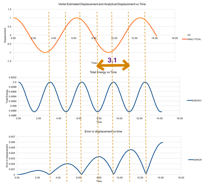
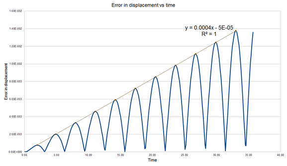
Tick. Nice figures. By estimating the maxima of the displacement error-time graph, the maxima were fitted against time. A very strong positive correlation was obtained from the fitting with a constant time interval of 3.1 in Figure 2, which allows us to predict time of the next maxima with its corresponding magnitude.

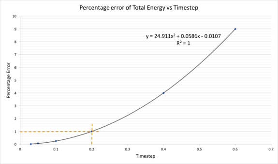
The percentage difference of energy from it's maxima (true value in SHM) was used to represent the percentage error of the total energy of the system. The relationship between the percentage error of the total energy and timestep was determined. The percentage error of the total energy increases with timestep. Therefore, the larger the timestep, the more deviated the system is from reality, and conservation of energy is disobeyed at large timestep. Any system with percentage error of total energy more than 1% is avoided, which give rise to the usage of timestep of less than 0.2. Tick. Correct tilmestep.

Figure 2: Error in the displacement of 1-D harmonic oscillator calculated from Verlet algorithm oscillates. The peak (local maxima) happens with a fix time interval (3.1 s for this case) and the magnitude of the local maxima varies linearly with time.

Figure 3: Plot of percentage error of the total energy vs timestep. By changing the timestep, the magnitude of the fluctuation of total energy of the system gets larger with larger timestep. Quadratic relationship between percentage error of the total energy and timestep was obtained.

Tick for figures

By monitoring the total energy of the system, the conservation of energy is ensured to satisfy the first law of thermodynamics. The less the fluctuation of the total energy of the system, the better the system is in describing the reality which is bounded by the first law of thermodynamics.

=== Analysing Lennard-Jones potential === Showing more working out would have been helpful for this section.

Figure 4: Comparison of a Lennard-Jones potential and Morse potentials with α scaled to fit the second derivative at the minimum (κ = 1), and obtained from fitting MP2 calculations (κ = 0.877).

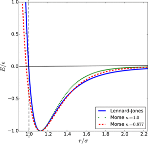
Lennard-Jones potential is used to estimate the interaction between particles in a simulation. It is a rough estimate of the pair interaction which most of the neutral atoms or molecules abide. The Lennard-Jones potential is described as:

$\varphi \left(r\right)=4ϵ(\frac{{\sigma }^{12}}{r^{12}}-\frac{{\sigma }^6}{r^6})$

where $ϵ$is the depth of the potential well, $\sigma$ is the finite distance at which the potential is zero and $r$ is the distance between particles.

Differentiating the equation gives,

${\varphi }^{\prime }\left(r\right)=4ϵ(-\frac{12{\sigma }^{12}}{r^{13}}+\frac{6{\sigma }^6}{r^7})$

which the negative of this represents the force, as $\mathbf{F}=-\frac{\mathrm{d}\varphi \left(\mathbf{r}\right)}{\mathrm{d}\mathbf{r}}$

At $r=\sigma$, Tick.

$\varphi \left(\sigma \right)=0$, ${\varphi }^{\prime }\left(\sigma \right)=4ϵ(-\frac{6}{\sigma })$, $\mathbf{F}=\frac{24ϵ}{\sigma }$ Tick.

The positive sign of the force suggests that the force is repulsive. The repulsive term dominates when $r$ gets closer to zero, and the equation diverges at $r=0$ due to the Pauli exclusion principle, which suggests that two particles could not be at the same space at the same time.

The equilibrium distance, $r_{eq}$ is defined as the distance which $\mathbf{F}=0$. Hence,

${\varphi }^{\prime }\left(r\right)=4ϵ(-\frac{12{\sigma }^{12}}{r^{13}}+\frac{6{\sigma }^6}{r^7})=0$

Which gives rise to $r_{eq}=2^{1/6}\sigma \approx 1.12\sigma$ Tick.

Well depth missing.

Integrating the potential gives,

$\int \varphi \left(r\right)\mathrm{d}r=4ϵ(-\frac{{\sigma }^{12}}{11r^{11}}+\frac{{\sigma }^6}{6r^5})$

As the equation converges at $r=\mathrm{\infty }$, the area under the curve gets smaller as $r$ gets larger. Therefore, when $\sigma =ϵ=1.0$,

$\underset{2\sigma }{\overset{\mathrm{\infty }}{\int }}\varphi \left(r\right)\mathrm{d}r=-0.02066$

$\underset{2.5\sigma }{\overset{\mathrm{\infty }}{\int }}\varphi \left(r\right)\mathrm{d}r=-0.006811$

$\underset{3\sigma }{\overset{\mathrm{\infty }}{\int }}\varphi \left(r\right)\mathrm{d}r=-0.002741$

These integrals are not correct.

In simulations, we define the cut-off point of the Lennard-Jones potential to ease the process of simulation as potential greater than the cut-off point is negligible.

For example, the Lennard-Jones parameters for argon are $$\begin{gathered} \sigma =0.34\mathrm{n}\mathrm{m},ϵ \\ / \\ {k}_B=120\mathrm{K} \end{gathered}$$.

If the LJ cutoff is $r^{*}=3.2$, this represents potential at $r>3.2\sigma =1.088\mathrm{n}\mathrm{m}$ is consider as zero.

The well depth of the potential is

$$\begin{gathered} ϵ=k_B\times 120\mathrm{K}\approx 0.9977{\mathrm{k}\mathrm{J} \\ \mathrm{m}\mathrm{o}\mathrm{l}}^{-1} \end{gathered}$$

and the reduced temperature, $T^{*}=1.5$ is

$T=1.5\times 120\mathrm{K}=180\mathrm{K}$ Tick

Simulation box

The number of particles in a small volume is still relatively large for computer to process. For example, 1 mL of water contains $3.346\times 10^{22}$ particles. For computer to simulate this amount of particles with their respective interactions will take ages. On the other hand, by simulating 10 000 water molecules, it only represents a volume of $2.99\times 10^{-19}$ mL Tick , which is too small to estimate bulk water. Therefore, the solution is to simulate 10 000 water molecules in a box and replicates $3.33\times 10^{18}$ boxes side by side to generate 1 mL of water. These boxes are bound to the periodic boundary conditions. Atoms leaving the box will reenter the box from the opposite side to conserve the number of atoms in the box. For example, an atom at position $(0.5,0.5,0.5)$ in a cubic simulation box which runs from $(0,0,0)$ to $(1,1,1)$ which moves along the vector $(0.7,0.6,0.2)$ will reenter the box from the opposite side and end up at position $(0.2,0.1,0.7)$. Tick

Moreover, initial positions of the particles are not given randomly in the simulation box because two particles might end up at the same position or positions which they are very close to each other. This case causes the particles to disobey the Pauli exclusion principle, or causes the initial potential between particles to be extremely large. As particles take up space, hard sphere model suggests particles as impenetrable spheres that cannot overlap in space. Therefore, particles initial positions are being set in a lattice space. Correct line of thought: assigning random coordinates can result in unphysically close atoms. However, you should always be aware of what model you are using - you have modelled particles as point masses, not hard spheres. It is impossible (ignoring how the computer stores your numbers here) for point masses to touch on a continues length scale them to actually "touch", so they never have the same coordinates. However, they can get very close, which would correspond to overlapping atoms in terms of their interactions. Overlapping atoms will likely cause the program to terminate with an error, but due to preset criteria that interpret the coordinates as unphysical. However (and more importantly) if these criteria are removed, and with a small enough timestep, the system will eventually equilibrate. This is of course unreasonably expensive, but we would be able to get to the equilibrated system starting from a configuration that is impossible with hard spheres.

Initially, particles are being arranged in lattice model such as simple cubic and face-centred cubic lattice, then they are allowed to move and reach equilibrium after some time. For example, the following LAMMPS input

lattice sc 0.8

generates simple cubic lattice with number density of 0.8. Since each unit cell in the simple cubic lattice has 1 atom, the volume of the unit cell must be 1.25, giving rise to the length of each side of the unit cell to be 1.077. For lattice fcc 1.2, each unit cell in the face-centred cubic lattice has 4 atoms, the volume of the unit cell is hence 3.33, giving rise to the side length of the unit cell to be 1.49 Tick . The following LAMMPS input

region box block 0 10 0 10 0 10

create_box 1 box

generates 10 unit cells in each of the x, y and z direction. Therefore, 1000 unit cells were generated, and 1000 atoms will be generated in simple cubic lattice, but 4000 atoms will be generated in face-centred cubic lattice Tick . The following LAMMPS input

mass 1 1.0
pair_style lj/cut 3.0
pair_coeff * * 1.0 1.0

specifies the mass of type 1 atoms as 1.0, with Lennard-Jones potential without Coulombic interaction between particles with a cutoff at

$r^{*}=3$

. Pairwise forcefield coefficients are specified in the script as well, with the asterisks representing all types of atoms with coefficients of 1.0 The "coefficients" are the finite distance (sigma) at which PE=0, and well depth (epsilon) . This command would mean that all atoms have the same affinity towards one another. Increasing the coefficients will simply means increasing the affinity of the molecules, increasing their interaction strength. Tick

After setting up the particles' initial positions and forcefield (which specifies particles' initial velocity), Verlet algorithm or Leapfrog integration could be used to estimate the consecutive particles' positions and velocities.

The following LAMMPS input,

### SPECIFY TIMESTEP ###
variable timestep equal 0.001
variable n_steps equal floor(100/${timestep})
timestep ${timestep}

### RUN SIMULATION ###
run ${n_steps}

define a new variable timestep, allowing us to change the timestep manually from the script. This variable is defined for convenience as it is called in the next line to compute the number of steps by itself from the timestep. Therefore, users do not need to change both the timesteps and the number of steps by themselves because the two of them are related, changing one of them will hence be sufficient. Tick

Equilibration

Figure 5: Total energy, temperature and pressure vs time graphs from simulation result for timestep of 0.001

From Figure 5, the system reaches equilibrium after some time, showing a constant fluctuation in the total energy, temperature and pressure. This constant fluctuation of total energy shows that the system has reached equilibrium and the fluctuation in the total energy could be explained from the error which origins from the Verlet algorithm as shown from the section above. In order to show the fluctuation has no positive or negative correlation (a constant straight line), the product moment correlation coefficient of the fitting of the later points is used.

Figure 6: Line fitting of the equilibrium region with the corresponding upper and lower limits and the comparison of the squared product moment correlation coefficient (PMCC) with the starting time used in the line fitting for timestep of 0.001.

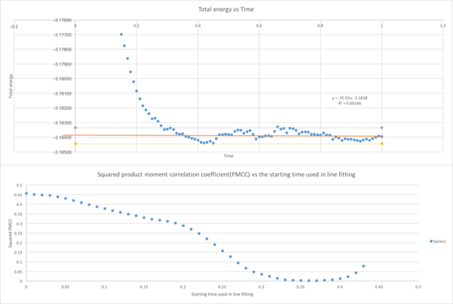
Figure 6 shows if all the points from the graphs were used in line fitting, a line with negative PMCC will be obtained, which explains the graph's negative correlation. When the starting time used for line fitting is at 0.36, the PMCC is closest to zero which shows no positive or negative correlation. This time is when the system reaches equilibrium. After 0.36, the PMCC rises again due to the slight positive correlation of the graph.

Figure 7: Total energy vs time graphs for different timesteps

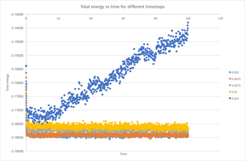
From Figure 7, 5 different timesteps were used in the simulation, but the largest timestep used, 0.015 shows a positive correlation instead of no correlation. Therefore, it is the worst choice of representation of reality because it does not reaches equilibrium, and the total energy diverges. This phenomenon could be explained from the error of the Verlet algorithm. Due to the nature of the Verlet algorithm which gives error while predicting the future value, when the timestep is sufficiently large, the error is too large, giving rise to larger error in the future values. You need to be more clear here. It's true that too large timesteps cause your system to become unstable; this arises from particles being "moved" to unrealistic places during trajectory propagation, and these unrealistic configurations have high PE. Indeed, the source of this "error" would be the velocity-verlet algorithm in your simulations, but it's a phenomena inherent to all integration schemes. The system hence move further and further away from the reality. The largest timestep from the 5 which gives acceptable result is 0.01, which is advantageous in observing the system for a long time using a short simulation time. The correct tilmestep was 0.0025 using the criteria specified in the task.

Appendix II- Sample of LAMMPS input in the NVE ensemble

variable density equal 0.2
variable temperature equal 2.0
variable timestep equal 0.002

lattice sc ${density}
region box block 0 15 0 15 0 15
create_box 1 box
create_atoms 1 box

mass 1 1.0
pair_style lj/cut/opt 3.0
pair_coeff 1 1 1.0 1.0
neighbor 2.0 bin

velocity all create ${temperature} 12345 dist gaussian rot yes mom yes

timestep ${timestep}
fix nve all nve

thermo_style custom step time etotal temp press
thermo 10

dump traj all custom 1000 output-1 id x y z

run 10000
unfix nve
reset_timestep 0

variable tdamp equal ${timestep}*100
fix nvt all nvt temp ${temperature} ${temperature} ${tdamp}
run 10000
unfix nvt
fix nve all nve
reset_timestep 0

thermo_style custom step atoms etotal temp vol density
variable temp equal temp
variable temp2 equal temp*temp
variable etotal equal etotal
variable etotal2 equal etotal*etotal
variable N2 equal atoms*atoms
fix aves all ave/time 100 1000 100000 v_temp v_etotal v_temp2 v_etotal2
run 100000

variable avetemp equal f_aves[1]
variable var equal (f_aves[4]-f_aves[2]*f_aves[2])
variable heatcap equal ${N2}*(${var}/f_aves[3])

print "Averages"
print "--------"
print "Ave Temperature: ${avetemp}"
print "Heat Capacity: ${heatcap}"

References

- ↑ H. Löwen, Computer Simulations in Condensed Matter Systems: From Materials to Chemical Biology Volume 2 Lecture Notes in Physics, 139–161.
- ↑ M. Levitt and A. Warshel, Nature, 1975, 253, 694–698.
- ↑ P. Šelepová and J. Kypr, Biopolymers, 1985, 24, 867–882.
- ↑ K. Aim, J. Kolafa, I. Nezbeda and H. L. Vörtler, Fluid Phase Equilibria, 1993, 83, 15–22.
- ↑ T. Nakagawa, Molecular Physics, 1996, 88, 1635–1644.
- ↑ S. V. Parter, Numerical methods for partial differential equations: proceedings of an advanced seminar conducted by the Mathematics Research Center, the University of Wisconsin, Madison, October 23-25, 1978, Acad. Press, New York, 1982.
- ↑ J.-P. Hansen and L. Verlet, Physical Review, 1969, 184, 151–161.
- ↑ P. W. Atkins, Shriver & Atkins inorganic chemistry, Oxford University Press, Oxford, 2010.
- ↑ Cengel, Yunus A.; Boles, Michael A. Thermodynamics: An Engineering Approach (4th ed.). p. 89. ISBN 0-07-238332-1.
- ↑ Y. A. Çengel and M. A. Boles, Thermodynamics: an engineering approach, McGraw-Hill Connect Learn Succeed, New York, 2011.
- ↑ D. Chandler, Introduction to modern statistical mechanics, Oxford Univ. Press, New York, NY, 2009.
- ↑ P. Flowers, K. Theopold, R. Langley, W. R. Robinson, M. Blaser, S. Bott, D. Carpenetti, A. Eklund, E. El-Giar, D. Frantz, P. Hooker, G. Kaminski, J. Look, C. Martinez, T. Milliken, V. Moravec, J. D. Powell, T. Sorensen and A. Soult, Chemistry, OpenStax, Rice University, Houston, TX, 2017.
- ↑ W. Brostow, Chemical Physics Letters, 1977, 49, 285–288.
- ↑ S. M. Lindsay, Introduction to nanoscience, Oxford University Press, Oxford, 2010.
- ↑ D. C. Wallace, Physical Review E, 1998, 58, 538–545.
- ↑ R. A. Serway and J. W. Jewett, Physics for scientists and engineers, Thomson/Brooks/Cole, Australia, 2004.
- ↑ T. C. O’Connor, J. Andzelm and M. O. Robbins, The Journal of Chemical Physics, 2015, 142, 024903.
- ↑ J. E. Jones, Proceedings of the Royal Society A: Mathematical, Physical and Engineering Sciences, 1924, 106, 463–477.
- ↑ P. Kosinski and A. C. Hoffmann, Physical Review E, 2011, 84.
- ↑ L. Verlet, Physical Review, 1967, 159, 98–103.
- ↑ J. Schmid, The Journal of Educational Research, 1947, 41, 311–313.