Rep:LSim:jw815

Overall Feedback. A generally good understanding of the MD simulations carried out was conveyed. The abstract, introduction and methodology sections were good. The results and discussion section would have benefited from being more concise: however this is difficult as some tasks were not appended at the end, but instead discussed in the report, increasing the length required to cover all the material. bbbutttt the lattice spacing for solids is in there! (and I didnt want to clutter some some workings with calculations that were leaning toward the basic side)  :( P.S I tried to structure some task in the results and discussion so that it could flow more appropriately like in a research paper, as was told to us. Yes, sorry I was thinking of the fcc lattice spacing, which you have included. I have edited the feedback accordingly, and you mark will of course reflect this. As for how a research paper should be written: as concisely as possible, with a clear motivation and logical progression. This is easier to do by first appending all the Q&A style tasks at the end (this appendix would not count as part of your report) so as to pick up all available marks there, and then selecting interesting parts of your results to write about in the report, so as to produce the highest quality report without having to worry about including information that may not be completely necessary to include. This is how we explained you should format your wiki page in the lab sessions.

Abstract

In this report, Molecular Dynamics Simulation (MDS) was used to study the diffusive and dynamic properties of different phases under varying thermodynamic conditions. The results obtained were largely consistent with our macroscopic understanding of these properties - the Radial Distribution Function (RDF) for the different phases is consistent with our understanding of microscopic structure of the phases, the diffusion coefficients calculated using the mean square displacement and velocity correlation function techniques showed characteristic behavior with ballistic and diffusive regimes. However, the limitations of simulations are also highlighted in these calculations, where deviation from expected behavior is observed.

Nice and concise. You could have included 1-2 sentences of motivation. It is not important, but molecular dynamics is usually abbreviated to MD; MDS for "molecular dynamics simulation" is rarely seen.

Introduction

MDS act as a bridge between microscopic length and time scales and the macroscopic world. By providing a guess of the interactions between particles, we obtain a prediction of the bulk thermodynamic properties. MDS also allows us to obtain hidden details behind bulk measurements, for example, the velocity autocorrelation function is linked to the diffusion coefficient, but the former is much easier to calculate computationally while the diffusion coefficient is much easier to obtain experimentally. MDS also has numerous real-world applications ranging from molecular biology, where it has been used to effectively to enhance our understanding of protein folding ion transport across membranes, and even in environmental studies to study the dehumidification process in air. More directly, the results obtained from this present study (e.g. in diffusion) is a starting point for more complex studies, such as in the diffusion of nanoparticles (NPs) through mucus layer in drug delivery systems.

I really like this introduction. Good points made using simple, easy to understand language. A bit more specificity would have been a bonus.

Aims and Objectives

• Demonstrate how a Lennard-Jones fluid can be simulated to provide information on bulk properties of systems that are weakly interacting (e.g. Ar). Such information include the density, heat capacity, structural properties, and diffusive properties.
• Highlight that bulk properties (e.g. diffusion coefficient) can be calculated using different methods
• To rationalise any differences observed between these simulations compared to (1) Ideal gas behaviour (2) Experimentally obtained results.

Simulation Method

All simulations were performed using the Large-scale Atomic/Molecular Massively Parallel Simulator Package (LAMMPS). Fluids were modelled using a Lennard-Jones potential with a cut-off radius of σ=3. Long tail correction was not applied in order to improve computational efficiency Nice detail, although we really could have afforded it, it's very cheap. . All Liquid and vapour phase simulations were melted from a simple cubic crystal (sc) with an input density of 0.8 and 0.01 respectively, whereas the solid phase was simulated with a face-centered cubic (fcc) lattice with an input density of 1.2. The use of a lattice avoids random generation of atoms which result in large energies being computed. Unless otherwise stated, the simulation was performed at T=1.2 and controlled using a thermostat and barostat. All thermodynamic quantities were recorded every 0.002fs time steps, and the data was processed using Microsoft excel You do not and should not have to credit excel. Your analysis could have been done in a variety of software packages, so this is not needed for reproducibility. This argument could sometimes be made for the simulation package (LAMMPS) used, however these sometimes contain subtleties in approximations/numerical methods that may not make them completely equivalent to other software packages. This is more prevalent in QM packages e.g. VASP vs. CP2K. Also, LAMMPS does a lot of work, so it's worth crediting (which you have done). . Unless otherwise stated, all data presented are in reduced units.

I could reproduce your results with these details - good. .

Results and Discussion

Density as a function of temperature

Figure 1: Density as a function of temperature at different pressures

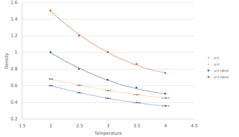
At both pressures, the simulated density is lower than the density as predicted by the ideal gas model. This is because the ideal gas model assumes that particles behave do not interact (in this context, they do not repel each other) and therefore more particles can fit into a confined space. However, in the simulated model, the atoms are governed by Lennard-Jones interactions. When the interatomic separation is small, the repulsion term dominates, and the atoms are pushed further apart from each other, resulting in a lower density.

As temperature increases, the deviation from ideal behaviour is less in both cases. This is because at high temperatures, particles oscillate about the equilibrium to a greater extent and this fast oscillation makes the interaction between particles transient (as they have no time to react to these interactions I understand what you are trying to say, but the wording makes it not completely correct. ). This is analogous to experiencing weaker interactions/repulsions and hence tending towards ideal behaviour. Analogues - yes, as in has the same effect (greater KE to overcome kinetic berries in the PES), but not the same. You could explain these points more clearly.

Comparing the simulations at higher and lower pressure, the one at higher pressure shows a greater deviation from ideality at all temperatures. This is a result of the greater interatomic interactions/repulsions by atoms which are found closer together at higher pressure.

Heat Capacity as a function of temperature

Figure 2: Heat capacity at constant volume as a function of temperature at different densities

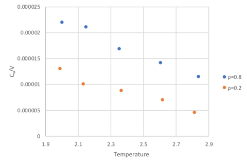
At both densities, heat capacity at constant volume decreases as temperature increases. At higher temperatures, higher energy states can be occupied resulting in an increase in the density of high energy states. Thus, less energy is required to bring about the same increase in temperature of a system compared to a system at lower temperature, where the states populated are low in energy. This trend is expected for real gases which experience interatomic interactions modelled by a Lennard-Jones potential. For a monoatomic ideal gas, with no interactions, the heat capacity corresponds to $C_V=\frac{3}{2}R$, which would be represented by a horizontal line with a constant value in the graph. There's a bit of a misunderstanding here - between the inherent chemical properties of a system and what changing these properties would mean for the heat capacity and simulating the heat capacity over our simulation of Lennard-Jones particles. In our simulation, and what I've tried to get people previously to suggest, we see a slight decrease in heat capacity with increasing temperature. What do we expect? Constant number of particles.. Internal enegy remains constant.. Cv = dU/dT and thus constant heat capacity. If I changed the material or the particles and changed the DOS or inherent properties of the systme, the heat capacity would vary as you suggest.

At higher density, the heat capacity is also higher. This is also expected because a system of higher density has more energy levels per unit volume, and more energy is required to effect the same increase in temperature. This is distinct from the temperature argument which is concerned with the relative population of states, rather than the the number of states per unit volume in the first place.

Furthermore deviations from expected constant behaviour can also be explained through simulation limitations. Specifically, a small LJ cut-off radii of σ=3 was chosen to improve computational efficiency. However, this results in a loss of long range interactions. Given that the values of C_V is small (10^-5 in magnitude), this potentially results in susceptibility to errors.

Radial Distribution Function

Figure 3: Radial Distribution Function (RDF) as a function of r for a simulated LJ solid, liquid, and gas. T=1.2 were used for the simulations and Solid(fcc, ρ =1.4), Liquid(sc, ρ =0.8), Gas(sc, ρ =0.01)

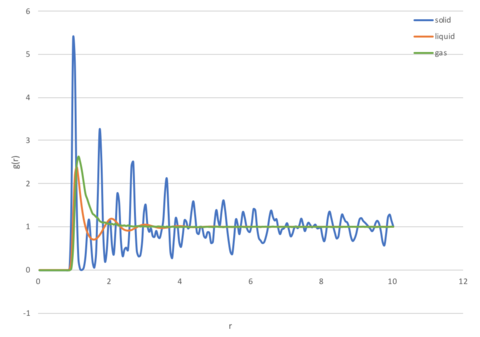
The Radial Distribution Function (RDF), $g(r)$, is the probability of finding a particle at distance $r$ from another tagged particle. This function correlates the bulk density of the matter, ${\rho }^{bulk}$ (which will always be constant) and the local density or number density, $\rho (r)$ (which is dependent on the distance $r$ from a reference point) according to equation 1.

$$\begin{gathered} \rho (r)={\rho }^{bulk}g(r) \\ (1) \end{gathered}$$

Solids

Figure 4: Positions of atoms in a fcc lattice, with the respective distance for each coordination shell shown

Solids have regular periodic structures as a result of short and long range interactions, with atoms vibrating about their specific lattice positions. The peaks observed (Figure 3) corresponds to where the atoms are highly likely to be found (in their lattice positions), for this simulation in a fcc lattice, the first, second, and third peak at σ, √2σ, √3σ corresponds to the first second third coordination shells respectively. These shells are illustrated in Figure 4, with atoms at position [0.5 0.5 0.5] contributing to the first shell, atoms at position [1 0 0] contributing to the second shell, and atoms at position [1 0.5 0.5] contributing to the third shell. The probability of locating an atom between peaks is very low, as the atoms are already packed very closely together to fill the space most efficiently.

Liquids

Atoms in liquid move dynamically and do not maintain a fixed structure. Their short range order is represented by the presence of peaks at small r, with the first peak at σ corresponding to the first coordination sphere, and the next one at an approximate distance of ~σ (approximate because there is no exact ordering in the liquid). The peaks eventually decrease in amplitude as long range order is lost, and at large r, the atoms are practically independent of each other and the distribution returns to g(r)=1. It is important to note that because a cut-off of 3σ was used in the simulation, no peaks are seen after this limit. In reality, it can be expected that small peaks will still be seen in the region where the separation does not preclude any interactions from occurring.

Gases

Gaseous atoms do not have an ordered structure, and will only show one broad peak initially, after which it plateaus at g(r)=1. This is because the atoms are moving around randomly in a sporadic motion (Brownian motion), and at most only have a single short-lived coordination sphere representing the interactions between particles at close range modelled by the Lennard-Jones potential used for this simulation. Once again, because a cut-off of 3σ was used, any potential interactions at this range were ignored.

Diffusion Coefficient

Method 1: Mean Squared Displacement

Figure 5: MSD against timestep for a solid system.

Figure 6: MSD against timestep for a liquid system.

Figure 7: MSD against timestep for a gaseous system.

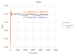
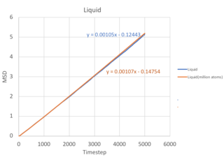
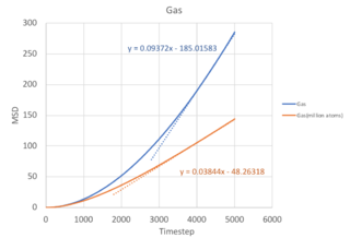
The Mean Square Displacement (MSD), $⟨r^2\left(t\right)⟩$, is a measure of the deviation of a particle with respect to a reference position over time. Mathematically, it is related to the diffusion coefficient through:

$$\begin{gathered} D=\frac{1}{6}\frac{\partial ⟨r^2\left(t\right)⟩}{\partial t} \\ (2) \end{gathered}$$

From equation 2, it follows that the more a particle travels, the greater it's MSD, and hence the higher the diffusion coefficient. For solids, the atoms vibrate in fixed lattice positions, giving a constant MSD. Liquids and gases are not confined to fixed lattice positions, therefore MSD increases with time. In both cases, a parabolic behaviour is observed. This is because the the path an atoms takes will be an approximate straight line with constant velocity (proportional to time squared) until it collides with its neighbour - this corresponds to the ballistic regime of the system. Only when it starts the collision process will its path start to resemble a diffusive process, represented by the linear behaviour. The ballistic regime is less apparent in the MSD for liquids because atoms are found closer together and quickly collide, transiting to the diffusive regime. However, in a gaseous system, the atoms are further apart and each atom takes a longer time before a collision, therefore the ballistic regime is more pronounced.

In calculating the diffusion coefficient, we disregard the ballistic dynamics and only use the gradient from the last 2000 timesteps corresponding to the diffusive regime. In equation 2, the

$\frac{\partial ⟨r^2\left(t\right)⟩}{\partial t}$

term corresponds to the gradient of the MSD vs timestep graph, with

$r(t)$

computed in terms of σ=0.34nm, and

$\partial t$

corresponding to a timestep of 0.002fs used in this simulation.

Table 1: Diffusion coefficients obtained from the gradient of the MSD vs timestep graphs

	Normal simulation			Million atom simulation
	Gradient	D (σ2 0.002fs-1)	D (cm2 s-1)	Gradient
Solid	1.45 x 10-8	2.41 x 10-9	2.79 x 10-6	8.00 x 10-8
Liquid	1.05 x 10-3	1.75 x 10-4	0.202	1.07 x 10-3
Gas	9.37 x 10-2	1.56 x 10-2	18.0	3.84 x 10-2

As the timestep for the million atom simulation is not known - the diffusion coefficient cannot be calculated. You should have been able to calculate the million atom MSD. However, there are a few salient points when comparing with the normal simulation. First, the MSD fluctuates to a smaller extent in the million atom system, allowing us to obtain a more accurate value for the diffusion coefficient. This is illustrated most clearly in the solid simulation, where a larger system size equilibrates at a constant MSD value with lesser fluctuations. Second, the trend of diffusion coefficients increasing when moving from solid to liquid to gas is consistent with that of the normal simulation, as decreasing density increases the distance between atoms and allows for a greater deviation of an atom from its initial position.

Method 2: Velocity Autocorrelation Function

Figure 8: VACF against timestep for solid, liquid, and gas

Figure 9: VACF against timestep for solid, liquid, and a 1D harmonic oscillator when w=1/2π

Figure 10: VACF against timestep for solid, liquid, and a gas for a million atom simulation

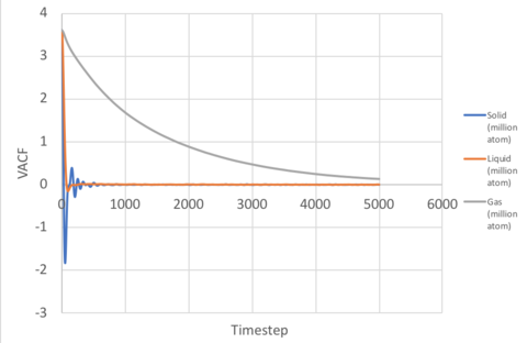
The Velocity Autocorrelation Function (VACF), $C(\tau )$, tells us how the velocity of an atom at time t, $\mathbf{v}(t)$ differs from its velocity at a different time, $\mathbf{v}(t+\tau )$. Mathematically, they are related through:

$$\begin{gathered} C\left(\tau \right)=⟨\mathbf{v}\left(t\right)\cdot \mathbf{v}(t+\tau )⟩ \\ (3) \end{gathered}$$

Integrating VACF then gives us the diffusion coefficient:

$$\begin{gathered} D=\frac{1}{3}\underset{0}{\overset{\mathrm{\infty }}{\int }}\mathrm{d}\tau ⟨\mathbf{v}\left(0\right)\cdot \mathbf{v}\left(\tau \right)⟩ \\ (4) \end{gathered}$$

Gas

In non-interacting systems a constant VACF is expected, as particles retain their velocity. If the interaction is weak but not negligible, then each atom would experience a gradual change in its magnitude and direction and slowly de-correlate with time. This explains the behaviour seen in a gas, where the VACF decreases steadily (Figure 8).

Solids and Liquids

If the interaction is strong, like in a solid or liquid, atoms tend to oscillate at the bottom of the LJ well where there is a balance between repulsive and attractive forces. This gives rise to the periodic oscillation from positive to negative values seen for solids (and very slightly for liquids). For solids, the atoms are held in fixed lattice positions and do not diffuse, therefore the oscillations are not dampened by diffusive motion (the dampening observed is due to other perturbative forces), however liquids do not have fixed positions and the atoms slide over each other frequently, and the diffusive motion results in a rapid disruption of the oscillatory behaviour, resulting in the VACF for the liquid decaying to zero after one minima.

1D Harmonic Oscillator

The VACF for a normalised harmonic oscillator in one dimension is given by (derivation in appendix):

$C\left(\tau \right)=\cos \left(\omega \tau \right)$

The VACF for the solid and liquid simulations are shown in Figure 9 together with the VACF for the harmonic oscillator when $\omega =\frac{1}{2\pi }$.

The magnitude of oscillation is constant and greater than that observed for both solid and liquid. This follows naturally from the oscillatory behaviour about the potential well, which is unaffected by perturbative forces, therefore no dampening is observed.

The minima of the VACF provides insight into the collision dynamics of the system. Mathematically, the minima relates to the maximum change in the magnitude or direction of atoms in the system. The physical interpretation of this is that the first minima corresponds to the time in which all the atoms in the system have collided at least once.

The diffusion coefficients were calculated from Equation 5, using the trapezeium rule to obtain the integrals, and summarised below:

Table 2: Diffusion coefficients obtained from the gradient of the VACF vs timestep graphs

	Normal simulation			Million atom simulation
	Area under Curve/Integral	D (σ2 0.002fs-1)	D (cm2 s-1)	Area under Curve/Integral
Solid	216.37	71.12	0.062	176.919
Liquid	233.96	77.99	0.067	155.586
Gas	12670.51	4223.50	3.65	4902.699

For the normal simulation, the trend is expected, although the diffusion coefficient for solid is much higher than what we would expect. For the million atom simulation however, the trend is anomalous, with the diffusion coefficient obtained for solid being higher than that for liquid. Like in the MSD case, the million atom simulation shows less fluctuation than the normal simulation, and a more accurate value of VACF is obtained. The largest source of error in the VACF estimate for the diffusion coefficient arise from the numerical method used to evaluate the integral. While the trapezium method provides a good estimate, values are lost in each step of the calculation. In addition, the VACF is a slowly decaying function, therefore the tail contributes a significant amount to the integral, increasing the inaccuracy of the value obtained.

Conclusion

MDS is a powerful tool that can be used to obtain important information about a system without having to run laboratory experiments. We have demonstrated how simple simulations of Ar atoms with interactions modelled by an LJ potential can allow us to study how the density or heat capacity of fluids change as function of temperature. The RDF has also been used to study the underlying structure of fluids, with results obtained in agreement with our understanding of lattice spacings, coordination spheres, and coordination numbers. Lastly, we have shown how MDS can be used to obtain the diffusion coefficients using the MSD and VACF, each method carrying their own advantages and disadvantages Briefly summarising these advantages/disadvantages in 1-2 sentences would be helpful here. The numerical result from these also highlight that simulations may not always provide perfectly accurate values 1-2 sentences to summarise exactly how the numerical results highlight this would be good ., and thus have to be reinforced by experimental results.

Overall succinct conclusion. A more specific summation of your results would be good. A brief outlook paragraph would be a bonus.

Appendix

Input script for NVT simulations (shown is simulation at T=2.0 ρ=0.2)

variable density equal 0.2
variable temperature equal 2.0
variable timestep equal 0.002

lattice sc ${density}
region box block 0 15 0 15 0 15
create_box 1 box
create_atoms 1 box

mass 1 1.0
pair_style lj/cut/opt 3.0
pair_coeff 1 1 1.0 1.0
neighbor 2.0 bin

velocity all create ${temperature} 12345 dist gaussian rot yes mom yes

timestep ${timestep}
fix nve all nve

thermo_style custom step time etotal temp press
thermo 10

dump traj all custom 1000 output-1 id x y z

run 10000
unfix nve
reset_timestep 0

variable tdamp equal ${timestep}*100
fix nvt all nvt temp ${temperature} ${temperature} ${tdamp}
run 10000
unfix nvt
fix nve all nve
reset_timestep 0

thermo_style custom step atoms etotal temp vol density
variable temp equal temp
variable temp2 equal temp*temp
variable etotal equal etotal
variable etotal2 equal etotal*etotal
variable N2 equal atoms*atoms
variable vol equal vol
fix aves all ave/time 100 1000 100000 v_temp v_etotal v_temp2 v_etotal2
run 100000

variable avetemp equal f_aves[1]
variable varetotal equal (f_aves[4]-f_aves[2]*f_aves[2])
variable heatcap equal ${N2}*(${varetotal}/f_aves[3])

print "Averages"
print "--------"
print "Ave Temperature: ${avetemp}"
print "Heat Capacity: ${heatcap}"
print "Volume: ${vol}"

VACF derivation for a 1D Harmonic Oscillator

$x=Acos(\omega t)$ $$\begin{gathered} \mathbf{v}=\frac{dx}{dt}=-A\omega sin(\omega t) \\ (5) \end{gathered}$$

Given that the normalised VACF is given by:

$$\begin{gathered} C\left(\tau \right)=\frac{\underset{-\mathrm{\infty }}{\overset{\mathrm{\infty }}{\int }}\mathbf{v}\left(t\right)\mathbf{v}(t+\tau )\mathrm{d}t}{\underset{-\mathrm{\infty }}{\overset{\mathrm{\infty }}{\int }}{\mathbf{v}}^2\left(t\right)\mathrm{d}t} \\ (6) \end{gathered}$$

Substitution of $(5)$ into $(6)$ gives:

$\begin{array}{rl}[rcl]C\left(\tau \right)& =\frac{\underset{-\mathrm{\infty }}{\overset{\mathrm{\infty }}{\int }}\mathbf{v}\left(t\right)\mathbf{v}(t+\tau )\mathrm{d}t}{\underset{-\mathrm{\infty }}{\overset{\mathrm{\infty }}{\int }}{\mathbf{v}}^2\left(t\right)\mathrm{d}t}\\ & =\frac{\underset{-\mathrm{\infty }}{\overset{\mathrm{\infty }}{\int }}(-\mathrm{A}\omega \sin \left(\omega t\right))(-\mathrm{A}\omega \sin (\omega t+\omega \tau ))\mathrm{d}t}{\underset{-\mathrm{\infty }}{\overset{\mathrm{\infty }}{\int }}{(-\mathrm{A}\omega \sin \left(\omega t\right))}^2\mathrm{d}t}\\ & =\frac{\underset{-\mathrm{\infty }}{\overset{\mathrm{\infty }}{\int }}\sin \left(\omega t\right)\sin (\omega t+\omega \tau )\mathrm{d}t}{\underset{-\mathrm{\infty }}{\overset{\mathrm{\infty }}{\int }}{\sin }^2\left(\omega t\right)\mathrm{d}t}\end{array}$

Expanding the second term in the numerator using trigonometric identities:

$\begin{array}{rl}[rcl]C\left(\tau \right)& =\frac{\underset{-\mathrm{\infty }}{\overset{\mathrm{\infty }}{\int }}\sin (\omega t)[\sin (\omega t)\cos (\omega \tau )+\sin (\omega \tau )\cos (\omega t)]\mathrm{d}t}{\underset{-\mathrm{\infty }}{\overset{\mathrm{\infty }}{\int }}{\sin }^2\left(\omega t\right)\mathrm{d}t}\\ & =cos(\omega \tau )+\sin (\omega \tau )\frac{\underset{-\mathrm{\infty }}{\overset{\mathrm{\infty }}{\int }}\sin (\omega t)cos(\omega t)\mathrm{d}t}{\underset{-\mathrm{\infty }}{\overset{\mathrm{\infty }}{\int }}{\sin }^2\left(\omega t\right)\mathrm{d}t}\\ & =cos(\omega \tau )+\sin (\omega \tau )\frac{\underset{-\mathrm{\infty }}{\overset{\mathrm{\infty }}{\int }}\frac{1}{2}\sin (2\omega t)\mathrm{d}t}{\underset{-\mathrm{\infty }}{\overset{\mathrm{\infty }}{\int }}\frac{1}{2}[\cos \left(2\omega t\right)-1]\mathrm{d}t}\\ & =cos(\omega \tau )+\sin (\omega \tau )\frac{\underset{-\mathrm{\infty }}{\overset{\mathrm{\infty }}{\int }}\sin (u)\mathrm{d}u}{\underset{-\mathrm{\infty }}{\overset{\mathrm{\infty }}{\int }}\cos \left(u\right)-1\mathrm{d}u}\\ \end{array}$

The integral $\frac{\underset{-\mathrm{\infty }}{\overset{\mathrm{\infty }}{\int }}\sin (u)\mathrm{d}u}{\underset{-\mathrm{\infty }}{\overset{\mathrm{\infty }}{\int }}\cos \left(u\right)-1\mathrm{d}u}$ will tend to zero, hence:

$C\left(\tau \right)=\cos \left(\omega \tau \right)$

Tick.

Misc. Questions

Introduction to Molecular Dynamics Simulation

Task 1: Velocity-Verlet Algorithm

Figure 11: (Top) Comparison between analytical displacement modelled by a harmonic oscillator and the Verlet estimated displacement (Middle) Total energy against time using the Verlet algorithm (Bottom) Error in Verlet algorithm compared to analytic model. Note: All graphs use timestep = 0.1

Figure 12: Error in Verlet algorithm compared to analytic model when the timestep used is increased. Shown here is timestep = 0.2

Using the velocity-Verlet algorithm to model the behaviour of the classic harmonic oscillator (Figure 1), we see a good fit between the analytical data modelled by the harmonic oscillator and the velocity-Verlet solution (top graph). The error, given by the absolute difference between the analytical result and that modelled by the velocity-Verlet solution, shows a series of maximums of increasing amplitude (bottom graph). The positions of the maxima in the error function can be linearly represented by the Equation 7, and shown in Figure 11.

$$\begin{gathered} \mathbf{y}=0.00042155\mathbf{x}-0.000073022 \\ (7) \end{gathered}$$

When the error is at a minimum value, it corresponds to a maximum energy value of 0.500, suggesting that the true energy value of the system is 0.500. In contrast, when the error is at a maximum, it corresponds to the minimum of the energy function - the exact value of the minimum will depend on the timestep used. When timestep is increased, the error maxima increase at a greater rate as compared to a lower timestep, resulting in a greater amplitude of fluctuation in the energy. This is illustrated in Figure 12, where a higher timestep of 0.2 results in greater fluctuation in energy. This vale is also is the maximum threshold to obtain an error in energy of less than 1%, where the energy (0.5) experiences a maximal fluctuation of 0.05. Correct, we are after the largest timestep that meets the stability criteria: this was 0.2.

It is important to monitor the total energy of a physical system when modelling its behaviour numerically because when a system has equilibrated, the total energy should remain constant, indicating that energy has been completely redistributed amongst the colliding particles in the system. This is not always the case. It's true that we monitor the energy as an indication of the system's "health" for this simulation: but why? Think about what ensemble you're in (microcanonical) and what quantities are conserved. Would you do the exact same thing for another ensemble, e.g. NTV?

Task 2: Atomic Forces

For a single Lennard-Jones interaction, $\varphi \left(r\right)=4ϵ(\frac{{\sigma }^{12}}{r^{12}}-\frac{{\sigma }^6}{r^6})$, when the potential energy, $\varphi$, is zero: $r_0$= $\sigma$, and force is at the regime where repulsion dominates. You should show your working out. You also forgot to calculate the force at $r_0$

The equilibrium separation, $r_{eq}$, occurs when the force is zero, i.e.

$\mathbf{F}=-\frac{\mathrm{d}U}{\mathrm{d}\mathbf{r}}=0$

$\frac{\mathrm{d}U}{\mathrm{d}\mathbf{r}}=-48ϵ{\sigma }^{12}(\frac{1}{r^{13}})+24ϵ{\sigma }^6(\frac{1}{r^7})=0$

$\frac{1}{r_{eq}^7}=2{\sigma }^6(\frac{1}{r_{eq}^{13}})$

$r_{eq}=2^{\frac{1}{6}}\sigma$

At $r_{eq}=2^{\frac{1}{6}}\sigma$, $\varphi \left(r_{eq}\right)=-ϵ$

The integral of the potential is given by:

$\int \varphi \left(r\right)\mathrm{d}r=4ϵ(-\frac{{\sigma }^{12}}{11r^{11}}+\frac{{\sigma }^6}{5r^5})$

When $\sigma =ϵ=1.0$, $\int \varphi \left(r\right)\mathrm{d}r=-4(\frac{1}{11r^{11}}-\frac{1}{5r^5})$. Hence

$\begin{array}{rlr}[rcl]\underset{2\sigma }{\overset{\mathrm{\infty }}{\int }}\varphi \left(r\right)\mathrm{d}r& =-4(\frac{1}{11\times 2^{11}}-\frac{1}{5\times 2^5})& \approx 0.0248\\ \underset{2.5\sigma }{\overset{\mathrm{\infty }}{\int }}\varphi \left(r\right)\mathrm{d}r& =-4(\frac{1}{11\times 2.5^{11}}-\frac{1}{5\times 2.5^5})& \approx 0.0082\\ \underset{3\sigma }{\overset{\mathrm{\infty }}{\int }}\varphi \left(r\right)\mathrm{d}r& =-4(\frac{1}{11\times 3^{11}}-\frac{1}{5\times 3^5})& \approx 0.0033\end{array}$ Tick

Task 3a: Periodic Boundary Conditions

Under standard conditions, water has a density of ρ = 1 g/mL and molar mass of water = 18.0153 g/mol. Therefore for 1 mL = 1 g of water, the number of moles of 1ml water = m/M_r = 0.0555084 mol, and the number of water molecules = nN_A = 3.343 x 10²².

For 10000 water molecules, n of water = 1.661 x 10^-20 mol, mass of water = nM_r = 2.992 x 10^-19 g. Hence volume of water = 2.992 x 10^-19 mL. Tick

Task 3b: Periodic Boundary Conditions

Final atom position = $(0.5,0.5,0.5)+(0.7,0.6,0.2)=(1.2,1.1,0.7)$

After applying periodic boundary conditions, any coordinate greater than 1.0 will be translated in the negative direction by 1.0, we end with coordinate = $(0.2,0.1,0.7)$ Tick

Task 4: Reduced Units

$r=r^{*}\sigma$

$r=3.2(0.34)(10^{-9})=1.088nm$

$\varphi (r_{eq})=ϵ=(k_{B}T)(N_A)=(1.38065\times 10^{-23})(6.022\times 10^{23})=997.73546\mathrm{J}\mathrm{m}\mathrm{o}{\mathrm{l}}^{\mathrm{-}\mathrm{1}}=0.998\mathrm{k}\mathrm{J}\mathrm{m}\mathrm{o}{\mathrm{l}}^{\mathrm{-}\mathrm{1}}$

$T=\frac{T^{*}ϵ}{k_B}=1.5\times 120\mathrm{K}=180\mathrm{K}$

Tick

Equilibration

Task 1: Creating a Simulation Box

In simulations, atoms which are generated by the random style may be highly overlapping, causing many interatomic potentials to be computed as large energies and forces which would blow atoms out of the simulation box, causing LAMMPS to return an error. This can be avoided by imposing a limit on the maximum distance an atom can movie in a single timestep by using the fix nve/limit command, this allows the system to equilibrate at the energy minimum. Alternatively, the positions of the atom can be pre-defined by a known lattice type before running the simulation to avoid the overlaps.

Tick. Good that mentioned what LAMMPS does. You could also remove the stability criteria, and use a very small tilmestep, but this is more expensive and more effort than it's worth... it is never done, but you should be aware why we can do this.

Task 2a: Lattice Types: simple cubic

Figure 13: Different lattice types with different arrangement of atoms within each unit cell.

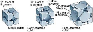
Different lattice types can be used to pre-define the position of atoms before a simulation. In these cubic lattice, the number density, $\rho =\frac{N}{V}$, where $N$ is the number of atoms per unit cell and the volume,$V=L^3$.

For example, in the simple cubic (sc), each unit cell contains $N=(\frac{1}{8})(8)=1$, if the number density, $\rho =0.8$: $L=\sqrt[3]{\frac{1}{0.8}}=1.07722$

When a box containing 1000 unit cells (and hence 1000 lattice points) is created, the create_atom function will generate 1000 atoms for the simulation, since each unit cell contains 1 atom

Tick

Task 2b: Lattice Types: face-centered cubic

For a face-centered cubic (fcc), each unit cell contains $N=(\frac{1}{8})(8)+(\frac{1}{2})(6)=4$, if the number density, $\rho =1.2$: $L=\sqrt[3]{\frac{4}{1.2}}=1.49380$

When a box containing 1000 unit cells (and hence 1000 lattice points) is created, the create_atom function will generate 4000 atoms for the simulation, since each unit cell contains 4 atoms.

Tick

Task 3: Properties of Atoms

After defining the position of the atoms, the properties were assigned using the following commands.

mass 1 1.0 
pair_style lj/cut 3.0
pair_coeff * * 1.0 1.0

mass 1 1.0: defines type 1 atoms as having a mass of 1.0

pair_style lj/cut 3.0: specifies a standard Lennard-Jones potential with no Coulomb between atom pairs, with global LJ cutoff set to distance $r=3.0$

pair_coeff * * 1.0 1.0: sets the pairwise forcefield coefficients for the symmetric I,J interaction to the same value of 1.0 for all (given by asterisk) type 1 with type 1 atom pairs the two ones correspond to the well depth and sigma

Tick

Task 4: Choice of Algorithm

Since the ${\mathbf{x}}_i\left(0\right)$ and ${\mathbf{v}}_i\left(0\right)$ will be specified in this simulation, the velocity-Verlet algorithm will be used. Tick

Task 5: Running a Simulation

Total time = timestep x number of timesteps. By defining the timestep and number of timesteps as a variable, we only need to change the timestep when running different simulations, and the number of timesteps will change correspondingly according to the formula to keep the total time constant. For the alternative input, which already specifies both timestep and number of timesteps, upon changing the timestep, we have to manually calculate the number of steps and input them for each different simulation to ensure that the total time remains the same. Tick

Task 6: Checking Equilibration

Figure 14: Total Energy, Pressure, and Temperature against time when a timestep of 0.001 is used. Time is shown up to 1s to illustrate the point of equilibration.

Figure 15: Total Energy against time when a timestep of 0.001 is used

Figure 16: Comparison of Total Energy against time at different timesteps

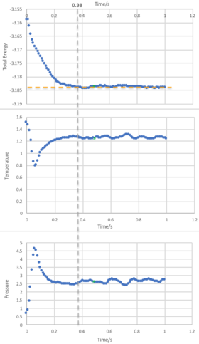
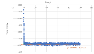
From Figure 15, we observe that an equilibrium energy value of -3.1482 is reached at a very early stage in the simulation with a timestep of 0.001. An expanded view showing the the first second of the simulation for the energy, temperature and pressure is shown in Figure 14, and it can be seen that equilibrium values are reached at approximately 0.38 seconds.

In simulations, shorter timesteps allow us to obtain more accurate calculations, although it can be costly and time-consuming to run such calculations. On the other hand, longer timesteps result in less accurate calculations. This balance is illustrated in Figure 16. When a long timestep of 0.015, the system stabilises at a minimum energy (at a value higher than the true vaue), but shortly after experiences a blowup as the errors start to propagate out of control, and therefore is a completely unacceptable timestep.

As the timestep decreases, an equilibrium is reached (0.01 and 0.0075), although it does not reach the true value of -3.184. Finally, as we further decrease the timestep to 0.0025, we see that a satisfactory value is obtained, which is identical to the most accurate value calculated at even lower timesteps. The balance in this simulation is thus to use a timestep of 0.0025, as it is high enough to avoid the high cost and time of simulations, yet low enough to obtain an acceptable calculation.

Correct choice of timestep for right reason. It would be good to add some intuition as to why larger timesteps cause the energy to diverge. Very large time steps will result in an unstable system. This line of reasoning would lead you to the rule of thumb that the tilmestep should be ~1/10 of the highest frequency mode.

Running Simulations under Specific Conditions

Task 1: Thermostats and Barostats

$$\begin{gathered} \frac{1}{2}\sum _i{m}_i{v}_i^2=\frac{3}{2}N{k}_{B}T \\ (8) \end{gathered}$$

$$\begin{gathered} \frac{1}{2}\sum _i{m}_i{\left(\gamma v_i\right)}^2=\frac{3}{2}N{k}_B\mathfrak{𝔗} \\ (9) \end{gathered}$$

As $\gamma$ is a constant, can be taken out of the sum in $(9)$ to give:

$$\begin{gathered} \frac{1}{2}{\gamma }^2\sum _i{m}_i{v}_i^2=\frac{3}{2}N{k}_B\mathfrak{𝔗} \\ (10) \end{gathered}$$

Substitution of $(8)$ into $(10)$

${\gamma }^2\frac{3}{2}N{k}_{B}T=\frac{3}{2}N{k}_B\mathfrak{𝔗}$

Cancelling out terms and rearranging gives:

$\gamma =\sqrt{\frac{\mathfrak{𝔗}}{T}}$

Task 2: Examining the Input Script

fix aves all ave/time 100 1000 100000 v_dens v_temp v_press v_dens2 v_temp2 v_press2

For the command ave/time, 100, 1000 and 100000 corresponds to Nevery, Nrepeat, and Nfreq respectively. These arguments specify on what timesteps the input values will be used in order to contribute to the average. Specifically, the final averaged quantities are generated on timesteps that are a multiple of Nfreq, and the average is over Nrepeat quantities, computed in the preceding portion of the simulation every Nevery timesteps.

To illustrate the code above, let value at each timestep $x$ denoted as $V_x$

Nevery=100 : Value is computed every 100 timesteps (i.e. $V_{100}+V_{200}+V_{300}+....)$

Nrepeat=1000 : Average will be over 1000 quantities (i.e. 1000 $V_x$ values)

Nfreq=100000 : Final averaged quantity is generated on timesteps that are a multiple of 100000

The Initial averages,

$A{V}_1=\frac{V_{100}+V_{200}+V_{300}+V_{400}...+V_{100000}}{1000}$

$A{V}_2=\frac{V_{100100}+V_{100200}+V_{100300}+V_{100400}...+V_{200000}}{1000}$

The Final averaged quantity, $AV=\frac{A{V}_1+A{V}_2+A{V}_3...+A{V}_n}{n}$

Because of the 'run 100000' at the end of the code, we are only dealing with 100000 timesteps, meaning that only $A{V}_1$ is taken since it already covers 100000 timesteps by itself. Assuming a timestep of 0.002fs, the simulation will take 0.002fs x 100000 = 200fs.

Tick.

Other tasks have been included in the write up.