Rep:LS:COH15

Abstract

Thermodynamic, structural and dynamical properties of solid, liquid and gase phase simulations modelled according to the Lennard-Jones potential were calculated on computational platform LAMMPS and VMD and discussed in this wikipage report. Density- temperature graph of simulation demonstrated the significance of inter-particle interaction and particle volume correction on Ideal Gas Law, and matches prediction in the Equation of state for substances in van der Waals force field. Heat capacity per unit volume - temperature graph further validate the expected behaviour of LJ lattice at temperatures above critical temperature. Experimental radial distribution function (RDF) confirmed that lattice type, spacing information, as well as other structure properties of gas, liquid and face centered cubic solid lattices matches with theoretical expectations. However, discrepency between theoretical ($1.494\sigma$) and experimental ($1.475\sigma \pm 0.05\sigma$) lattice spacing for FCC lattice raised attention to accuracy optimisation in future experiment. Diffusion coefficient at different phases were analysed using 2 different methods - the mean squared displacement and velocity autocorrelation function. Both methods produce similar results agreeing with theoretical expectations and differences in physical implications of each method were described.

Introduction

Molecular dynamic simulation is an important analytical tool allowing quick predictions of an experimental setting and validation by comparing with theoretical expectations. This technique can be applied to a wide range of research fields, from drug discovery to material engineering. One of the example would be the investigation of force field and crystal structure of RNA in its functional state to understand its role and working mechcanisms in biological processes, like DNA replication. In this experiment, various calculation and analytical tasks on the density-temperature-pressure relationship, heat capacity, radial distribution function, mean squared displacement, velocity autocorrelation function and diffusion coefficient of a Lennard-Jones model simulation were performed and discussed.

Aims and Objectives

A model of Lennard-Jones (LJ) fluid was simulated to provide insight to physical, structural and dynamical properties of systems with only weak van der Waals inter-particle interactions, one similar to that of Argon, at solid, liquid and gas phases. Structural properties, heat capacity, radial distribution function, mean squared displacement and diffusion coefficient of simulated systems were calculated in LJ reduced units and compared with theoretical expectations and reseults of a higher accuracy simulation.

Methods

Equilibrated Lennard-Jones fluid of well-depth, $ϵ$, and zero-potential inter-particle distance, $\sigma$, equaling to $1.0$ was constructed from the melting of a simple cubic lattice. Thermodynamc properties of systems were monitored, using state of the art software packages, up to a inter-particle distance cut-off of 3.0$\sigma$ for better computational efficiency. Timestep size of 0.0025 fs^-1 or 0.0020 fs^-1 was set to give the best balance between short simulation runtime and high accuracy. Reasoning for the selected timestep was explained in the appendix section.

Equation of State

2 sets of simulations were executed at $T^{*}=1.5,2.0,2.5,3.0,3.5,4.0,4.5,5.0,5.5,6.0,6.5,7.0,8.0and9.0$ under pressure of 1.0 and 2.0. Temperature and pressure of simulation were controlled by a thermostat and a barostat to ensure simulation is in the NpT ensemble. After performing 100000 runs per simulation, a final averaged quantity of density, temperature and pressure were calculated from the average of 1000 averaged values of every 100 repeats, as well as the corresponding standard error values. Density $(\frac{N}{V})$ against temperature plot at both pressure conditions were compared to the Ideal Gas Law and vand der Waals equation of state.

Heat Capacity

Heat capacity values of fluid at densities of 0.2 and 0.8 were measured at $T^{*}=2.0,2.2,2.4,2.6and2.8$. For this section of the experiment, simulations were changed to the NVT realm and brought to the desired state once an equilibrated fluid was created. Thermostat setting was disabled. In each simulation, average temperature and heat capacity values were printed at the end of the data file. Heat capacity values were calculated using the equation:

$C_V=\frac{\partial E}{\partial T}=\frac{\mathrm{V}\mathrm{a}\mathrm{r}\left[E\right]}{k_B{T}^2}=N^2\frac{⟨E^2⟩-{⟨E⟩}^2}{k_B{T}^2}$

where $\mathrm{V}\mathrm{a}\mathrm{r}\left[E\right]$ is the variance in $E$ and $N$ is the number of particles. Since energy values output from the simulation is divided by the number of particles $N$, the variance is multipled by a factor of $N^2$. $C_V/V$, where$V$ is the volume of the lattice, was plotted against $T^{*}$.

Structural Properties and Radial Distribution Functions

Trajectory data of simulations at gas, liquid and face centered cubic solid states were collected and used to calculate radial distribution function, $g(r)$, and $\int g(r)\mathrm{d}r$ of the systems. RDF graphs were analysed to give structural information of the systems. The density and temperature conditions of each states were as follows:

States	Lattice Type	Density	Temperature
Solid	FCC	1.2	0.5
Liquid	SC	0.8	1.0
Gas	SC	0.05	1.5

Dynamical Properties and Diffusion Coefficient

Mean squared displacement data was collected from simulations of the systems stated in the table below. According to the equation,

$D=\frac{1}{6}\frac{\partial ⟨r^2\left(t\right)⟩}{\partial t}$

$D$, the diffusion coefficient could be calculated fromm the gradient of the time-dependent mean squared displacemet function. Linear region of the funtion was fitted to get the gradient value along with its standard error.

States	Lattice Type	Density	Temperature
Solid	FCC	1.2	0.5
Solid	SC	1.2	1.2
Liquid	SC	0.8	1.2
Gas	SC	0.08	1.5

Velocity Auctocorrelation Function (VACF) of the above states, except for SC solid phase, were plotted againist time and analysed.

Results and Discussion

Equation of State

Figure 1. Density against temperature at pressure of 0.1 and 0.2

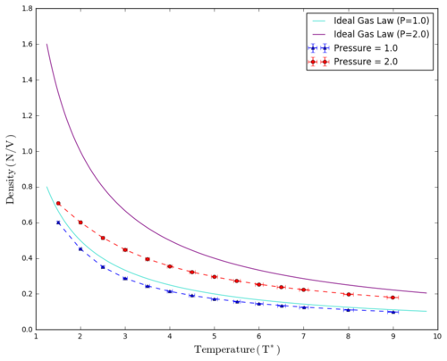
According to the van der Waals Equation of State:

$[P+a(\frac{N}{V}{)}^2](\frac{V}{N}-b)=k_{B}T$

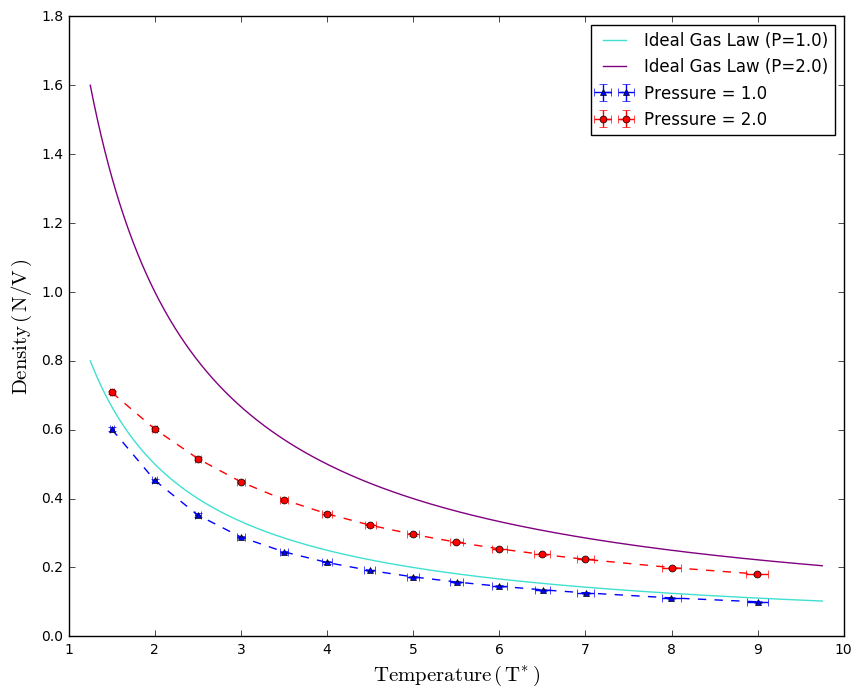
, where constant $a$ is an indication of inter-particle interaction and $b$ is an indication of particle volume. It is expected that density values of our simulations would be lower than the prediction of Ideal gas Law due to the fact that particle volume was accounted for in the vdW equation of state. It was noted that the difference between the experimental and theoretical values is greater at higher pressure than that at lower pressure due to the fact that the volume occupied by particles becomes more significant compared to the space between them. Similarly, the discrepancy decreases with temperature as at lower temperature, the system occupies a smaller volume, thus amplifying the effect of the coefficient $b$.

Error bars of both pressures at each temperature point is similar. Error bar for density values was so small that it is barely observable on the plot, indicating the repeats in each data point agrees with each other, showing that equilibrium is well reached in each run. It was also observed that error bar width of temperature values increases with temperature. This is probably due to the greater degree of lattice expansion at higher temperatures and therefore causing data points to deviate more fromm the maen value.

Heat Capacity

For a monoatomic ideal gas, kinetic energy of particles is the only contribution to internal energy of system, which gives a constant heat capacity value of $\frac{3k_B}{2}$ with no temperature dependence. However, in our LJ model, deviations from perfect gas behaviour was observed. Firstly, heat capacity per unit volume is greater at higher density. This is because of the increased amount of energy required to bring more particles per unit volume to a higher energy state in a denser substance. Also, higher density limits the degree of freedom of the system, so more energy is required. In the graph, heat capacity value also decreases with temperature. This is because at higher temperature, density of states increases, making it easier to promote atoms to higher energy level. The possible source of error is the loss in long-range van der Waals interactions beyond the cut-off at $3\sigma$.

Figure 2. Heat capacity per unit volume against temperature at density of 0.2 and 0.8

Structual Properties and Radial Distribution Function

Figure. 3 Radial Distribution Function Plot

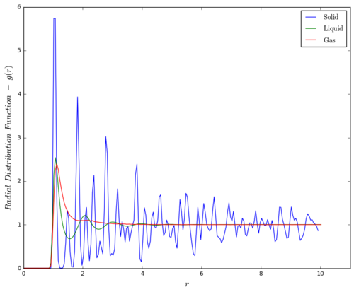
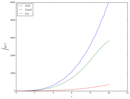
The radial distribution function (RDF), $g(r)$, is shown in Figure 3. Oscillating patterns are observed for face-centered cubic solid lattice and liquid phase, where as for gas phase, only one bread peak occured at 1.125$\sigma$ and then levels out to $g(r)=1$. This shows that gas phase of the fluid has no long or short-range order, where distribution of particles is effectively random at distance beyond the first shell of nearest neighbour, which held by weak van der Waals force. This analysis on different phases of different materials could be useful in identifying the effective range of a certain inter-particle interaction under different density and temperature conditions.

For liquid phase, a few periodic pattern was obesrved, but soon after that, the distribution approaches one. This shows that the liquid phase has some short-range order, but not as much as in solid phase. The peaks in liquid phase are broader than that of solid phase due to the fact that liquid particles do not have strict regularity in its configuration. Instead, successive coordination spheres are formed, where each particle is coordinated to multiple particles over a short range of inter-particle distance.

For the FCC solid crystal, sharp periodic spikes were oberved due to the fact that particles are in a fixed regular configuration in the lattice. Long-range order characteristic of solid phase is observed in the RDF plot. The first 3 nearest neighbour particles can be found at $r=1.025\sigma ,1.475\sigma ,and1.825\sigma$, corresponding to particles at $[\frac{1}{2}\frac{1}{2}\frac{1}{2}],[100]and[1\frac{1}{2}\frac{1}{2}]$ in the lattice. Lattice spacing of the simulated lattice equals to $r_2(i.e.1.475\sigma )$. This value is slightly smaller than the theoretical value of $1.494\sigma$ calculated in one of the Labbook tasks, but considering that there are actually 2 data points in the first peak, the actual experimental value of our first peak would lie between $1.475\sigma$ and $1.525\sigma$, agreeing with the theoretical value.

Figure. 4 Radial Distribution Function Plot of SC Lattice

In this section, lattice type of solid phase is modified to FCC instead of simple cubic (SC). It is because SC lattice gives a smooth RDF similar to that of a liquid but with greater amplitudes.(Figure 4) This result is probably caused by the melting of SC lattice. By changing lattice type to FCC, lattice density increases and limiting degrees of freedom the system, so that melting of lattice would not occur when crystal is being set to the desired conditions.

Dynamical Properties and Diffusion Coefficient

Mean Squared Displacement

Mean squared displacement (i.e. $⟨r^2(t)⟩$) is a measure of how much on average particles in the simulated state could travel from or vibrate about its equilibrium position. $\frac{\partial ⟨r^2(t)⟩}{\partial t}$ could therefore provide an indication of the mobility and thus diffusion coefficient of particles at a given phase. The mean squared displacement value of all phases are plotted and gradients of best fit lines at linear regions were used to calculate diffusion coefficient values, using the equation:

$D=\frac{1}{6}\frac{\partial ⟨r^2\left(t\right)⟩}{\partial t}=\frac{gradient}{6\times timestep}$

where the timestep for these simulations was 0.002 fs. In this simulation, FCC lattice was used for solid phase due to same reason as mentioned above.

Figure. 5 Mean Squared Displacement VS Time - Gas

Figure. 6 Mean Squared Displacement VS Time - Liquid

Figure. 7 Mean Squared Displacement VS Time - Solid Face Centered Cubic

In Figure 5, it is observed that the mean square displacement values for gas phases started with a ballistic superdiffusion region, where $⟨r^2(t)⟩\propto {\tau }^{\alpha }$ with $\alpha >1$. As time further increases, a linear relationship was observed. The ballistic region at the beginning is due to the fact that most particles are having random walks at slow initial velocity, allowing particles to travel further before encountering other particles in the system. As a result, diffusion coefficient for gas phase increases with time until equilibrium is reached. In Figure 6, the MSD plot for liquid is linear throughout the entire simulation, with small wavey fluctuations that can barely be seen along the trend. Looking at the MSD of solid, there is an initial spike and then the plot levels off with fluctuations about the average value. The spike is caused by competing attractive and replusive forces between paticles when the lattice is first created. As more time was given, the potential energy transforms into kinetic energy, where particles vibrate about their equilibrium position. Both liquid and solid phases shows damped oscillation pattern.

Comparing the gradients of the linear region for gas phase is much steeper than that in liquid and also solid phase, which is almost flat. This trend matches with our expectation as in gas phase, particles are the furthest away and therefore empty space between particles is significantly larger than particle size and the motion of gas particles has a lower chance of being interrupted by collisions or pairing interactions with surrounding particles, resulting in the highest diffusion coefficient. In liquid, particles are held closer together and higher probability for particle motions being hindered by van der Waals interactions and collisions with the surrounding particles, yielding a smaller diffusion coefficient value closer to that of a solid than gas particle. The diffucsion coefficients calculated agree wth our expectations as it is sensible that in regularly packed solid, particles has the least mobility to move about their equilibrium position giving the smallest diffusion coefficient.

Figure. 8 Mean Squared Displacement VS Time - Solid Simple Cubic

Figure 8 shows the mean squared displacement graph of the SC lattice. It is observed that the graph sttarted off with similar trend as a FCC solid crystal, with sharp increase in MSD at the beginning. However as time increases, the distribution function developed into a linear relationship, showing that particles in the SC solid state are no longer held tightly in place with rergular configuration. Instead, the graph shows the transition of a melting lattice from solid phase to liquid phase.

Figure. 9 MSD plot of 1 million atom simulations

Similar data analyis procedures were performed to the given data of a 1 million atom simulation mode in all phases. The plots and diffusion coefficient values of both sets of simulations gives the same trends and behaviours.

$State$	$Gradient$	$D/{\sigma }^2(0.002fs{)}^{-1}$	$D/c{m}^2{s}^{-1}$	$D(1million)/c{m}^2{s}^{-1}$
Solid - FCC	4.85e-08	8.09e-09	4.67e-06	1.41e-06
Solid - SC	4.50e-06	7.50e-07	4.33e-04	1.41e-06
Liquid	1.03e-03	1.72e-04	0.0994	0.101
Gas	0.0250	0.00417	2.41	3.63

Velocity Autocorrelation Function

The velocity autocorrelation frunction (VACF), $C\left(\tau \right)=⟨\mathbf{v}\left(t\right)\cdot \mathbf{v}(t+\tau )⟩$, measures the time-dependence of particle velocity in the system. Considering a system consist of a single atom with a given initial velocity, the particle following the Newtonian Law should return a flat horizontal VACF graph all time. In another words, the VACF plots could provide insights to the effects of particle collisions to the velocity of particles, as well as indications to the diffusion coefficient of the system through the equation:

$D=\frac{1}{3}\underset{0}{\overset{\mathrm{\infty }}{\int }}\mathrm{d}\tau ⟨\mathbf{v}\left(0\right)\cdot \mathbf{v}\left(\tau \right)⟩$

The normalised velocity autocorrelation function for a 1D harmonic oscillator was found to be $C(\tau )=\cos (\omega \tau )$ with workings provided in the appendix section.

Figure. 10 Plot showing Velocity Autocorrelation Function (VACF) of the 1 million atom simulation.

Figure. 11 Plot showing Velocity Autocorrelation Function (VACF) of the experiment simulation.

Above shown are the VACF graphs of the experimental simulation (Figure 11) and 1 million atom simulation (Figure 10) at all phases. Similar trends were observed in both graphs for each phase. For gas phase, velocity decorrelates with time as the gradual exponential decay in $C(\tau )$ shows that magnitudinal and directonal changes in particle velocity under the influence of weak van der Waals forces. The VACF approaches zero as gas particles reach the randomness at equilibrium state. Velocity-time decorrelation was also observed in liquid and solid phases. Damped oscillations is observed in solid phase. The sharp changes in velocity happened as a result of particles aiming to find a balance between the attractive and repulsive forces at restricted positions in the lattice. Particles therefore can only vibrate in their fixed position. Uneven oscillations are still observable even after some duration in the experiment simulation, unlike that of the 1 million atom simultaion. This is due to the presence of perturbative forces, disrupting the perfect oscillatory motion of solid particles. With longer time period given the uneven oscillation would decay to zero. As shown in the equation above, diffusion coefficient can be interpreted from the area under the VACF graph using trapezium rule. The calculated value of our simulation is expected to be lower than true value due to the cut-off conodition of long-range interactions over distance greater than $3\sigma$.

Conclusion

In conclusion, a LJ model at vapour, liquid and solid phases were simulted. From calculations and information collected, various trends and characteristics of the LJ model were observed. However, prior to carrying out calculations, conditions and assumptions of simulation was established. The velocity Verlet algorithm is used with periodic boundry condition applied. LJ coefficients, $\sigma$ and $ϵ$ were set to equal to 1. Reduced units were introduced to the simulation. Energy, pressure and temperature analysis were performed to find the optimal timestep of 0.0025. (Please refer to Lab Book tasks for detail description) Density-temperature graph in NpT ensemble shows small density value than predicted by Ideal Gas Law. Discrepency between experimental value and Ideal Gas Law expectation increases with pressure and decreases with temperature. Dominating contribution from particle volume to density of system was noted. Heat capacity per unit volume was noted to be higher at higher density and lower temperature. Experimental radial distribution function confirmed lattice type, spacing information, as well as other structure properties of gas, liquid and face centered cubic solid lattices matches with theoretical expectations. However, discrepency between theoretical ($1.494\sigma$) and experimental ($1.475\sigma \pm 0.05\sigma$) lattice spacing for FCC lattice raised attention to accuracy improvements in future experiment. Diffusion coefficient values generated from experimental MSD data agrees with that of the 1 million atom simulation. Although the some sections of our experimental results deviates from the Ideal Gas Law prediction, but it agrees with the Equation of states as well as the expectaing trends for a real fluid in LJ model. Through comparing MSD and VACF graphs of experimental results and the 1 million atom simulation, room for improvements in error minimisation are available to optimise our present simulation model. Larger lattice size means larger sample size and giving more reliable and accurate results. Introducing higher-order correction to calculation algorithm could improve accuracy of simulation.

References

[1] 1. E. A. Algaer, F. Müller-Plathe, Molecular Dynamics Calculations of the Thermal Conductivity of Molecular Liquids, Polymers, and Carbon Nanotubes. Soft Materials. 10, 42–80 (2012).

[2] Hansen, J. P., & Verlet, L. (1969). Phase transitions of the Lennard-Jones system. Physical Review, 184(1), 151–161. https://doi.org/10.1103/PhysRev.184.151

[3] Atkins, P., & De Paula, J. (2014). Physical Chemistry. In Atkins Physical Chemistry, 602-608.

Appendix: Lab Book

Introduction to molecular dynamics simulation

TASK:Open the file HO.xls. In it, the velocity-Verlet algorithm is used to model the behaviour of a classical harmonic oscillator. Complete the three columns "ANALYTICAL", "ERROR", and "ENERGY": "ANALYTICAL" should contain the value of the classical solution for the position at time $t$, "ERROR" should contain the absolute difference between "ANALYTICAL" and the velocity-Verlet solution (i.e. ERROR should always be positive -- make sure you leave the half step rows blank!), and "ENERGY" should contain the total energy of the oscillator for the velocity-Verlet solution. Remember that the position of a classical harmonic oscillator is given by $x\left(t\right)=A\cos (\omega t+\varphi )$ (the values of A, $\omega$, and $\varphi$ are worked out for you in the sheet).

TASK:For the default timestep value, 0.1, estimate the positions of the maxima in the ERROR column as a function of time. Make a plot showing these values as a function of time, and fit an appropriate function to the data.

TASK:Experiment with different values of the timestep. What sort of a timestep do you need to use to ensure that the total energy does not change by more than 1% over the course of your "simulation"? Why do you think it is important to monitor the total energy of a physical system when modelling its behaviour numerically?

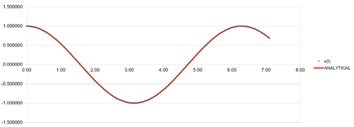
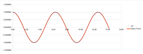
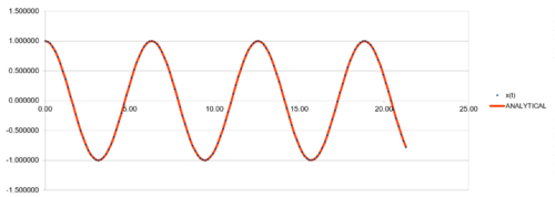
The velocity Verlet algorithm is tested against the "ANALYTICAL" (i.e. $x\left(t\right)=A\cos (\omega t+\varphi )$), calculated from the provided initial parameters (including force constant $(k=1)$, mass $(m=1)$, $A(=1)$, $\omega (=1)$ and $\varphi (=0)$) at 4 different timesteps. The absolute difference between "ANALYTICAL" and $x(t)$ (i.e."ERROR") were analysed. "ENERGY" values $(=\frac{k{x}^2+m{v}^2}{2})$ of classical harmomnic oscillator were also calculated from the $x(t)$,$v(t)$ and $F(t)$ values generated from the Verlet algorithm. The displacement plots showed periodic sinusoidal pattern every 2$\pi$ period between -1 and +1. Greater timestep gives longer period of simulation runtime with the same number of data points. The calculated values followed the analytical pattern tightly at all 4 timestep sizes tested, proving that the algorithm is a valid method to calculate particle behaviour. In addition, the energy plot does not show any sign of energy divergence, confirmed the calculation is valid and implemented correctly. The energy plot also show periodic behaviour with period of $\pi$. It is observed that amplitude of energy plots increases with timestep, showing that fluctuations in energy values beceome greater as step size increases.

Fig. 12 Position Plot - Timestep 0.05	Fig. 13 Energy Plot - Timestep 0.05	Fig. 14 Error Plot - Timestep 0.05
Fig. 15 Position Plot - Timestep 0.10	Fig. 16 Energy Plot - Timestep 0.10	Fig. 17 Error Plot - Timestep 0.10
Fig. 18 Position Plot - Timestep 0.12	Fig. 19 Energy Plot - Timestep 0.12	Fig. 20 Error Plot - Timestep 0.12
Fig. 21 Position Plot - Timestep 0.15	Fig. 22 Energy Plot - Timestep 0.15	Fig. 23 Error Plot - Timestep 0.15

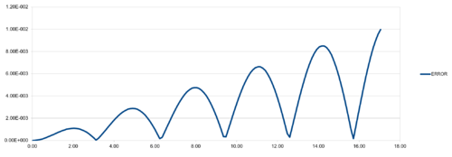
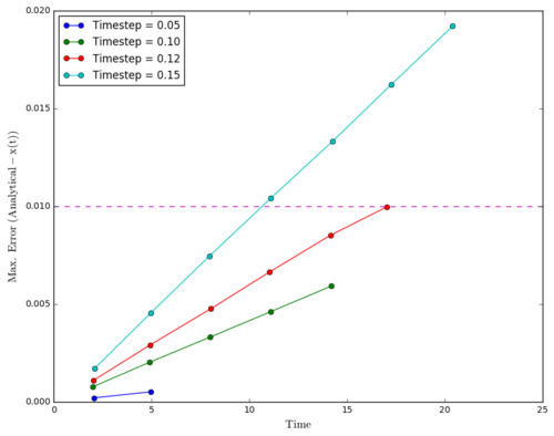
Regarding the difference between "ANALYTICAL" and calculated $x(t)$ values, amplifying periodic patterns were observed. Maxima of each loop were selected and plotted as shown in Figure 13. It is observed that error values increases with timmestep and length of simulation runtime. The acceptable timestep that satisfy within 1% error is 0.12(max. percentage error is 0.96%).

Fig. 24 Error Maxima Plot at 4 Different Timesteps

TASK: For a single Lennard-Jones interaction, $\varphi \left(r\right)=4ϵ(\frac{{\sigma }^{12}}{r^{12}}-\frac{{\sigma }^6}{r^6})$, find the separation, $r_0$, at which the potential energy is zero. What is the force at this separation? Find the equilibrium separation, $r_{eq}$, and work out the well depth $(\varphi \left(r_{eq}\right))$. Evaluate the integrals $\underset{2\sigma }{\overset{\mathrm{\infty }}{\int }}\varphi \left(r\right)\mathrm{d}r,\underset{2.5\sigma }{\overset{\mathrm{\infty }}{\int }}\varphi \left(r\right)\mathrm{d}r$, and $\underset{3\sigma }{\overset{\mathrm{\infty }}{\int }}\varphi \left(r\right)\mathrm{d}r$ when $\sigma =ϵ=1.0$.

Finding $r_0$, where $\varphi (r_0)=0$ :

$\varphi \left(r_0\right)=4ϵ(\frac{{\sigma }^{12}}{r^{12}}-\frac{{\sigma }^6}{r^6})=0$

$(\frac{\sigma }{r_0}{)}^{12}=(\frac{\sigma }{r_0}{)}^6$

$\sigma =r_0$

$\because Force=-\frac{\mathrm{d}\varphi \left(r\right)}{\mathrm{d}r}$

$\therefore Force=-4ϵ(\frac{-12}{r_0}+\frac{6}{r_0})=\frac{24ϵ}{r_0}$

Finding $r_{eq}$, where $\varphi (r_{eq})$ is at its minimum:

$\frac{\mathrm{d}\varphi (r_{eq})}{\mathrm{d}r}=4ϵ(-12(\frac{{\sigma }^{12}}{r^{13}})+6(\frac{{\sigma }^6}{r^7}))=0$

$2(\frac{{\sigma }^{12}}{r_{eq}^{13}})=(\frac{{\sigma }^6}{r_{eq}^7})$

$r_{eq}^6=2{\sigma }^6$

$\therefore r_{eq}=2^{1/6}\sigma$

$\varphi (r_{eq})=4ϵ(\frac{{\sigma }^{12}}{4{\sigma }^{12}}-\frac{{\sigma }^6}{2{\sigma }^6})$

$\therefore \varphi (r_{eq})=4ϵ(\frac{-1}{4})=-ϵ(i.e.welldepth)$

Evaluating icntegrals:

$\because \int \varphi \left(r\right)\mathrm{d}r=4ϵ[\frac{{\sigma }^{12}}{-11r^{11}}-\frac{{\sigma }^6}{-5r^5}]$

$Given\sigma =ϵ=1.0:$

$\underset{2\sigma }{\overset{\mathrm{\infty }}{\int }}\varphi (r)\mathrm{d}r=0-4[\frac{1}{5(2^5)}-\frac{1}{11(2^{11})}]=-0.0248(to3sig.fig.)$

$\underset{2.5\sigma }{\overset{\mathrm{\infty }}{\int }}\varphi \left(r\right)\mathrm{d}r=0-4[\frac{1}{5(2.5^5)}-\frac{1}{11(2.5^{11})}]=-8.18\times 10^{-3}(to3sig.fig.)$

$\underset{3\sigma }{\overset{\mathrm{\infty }}{\int }}\varphi \left(r\right)\mathrm{d}r=0-4[\frac{1}{5(3^5)}-\frac{1}{11(3^{11})}]=-3.29\times 10^{-3}(to3sig.fig.)$

It is observed that the integral value gets significantly small for $r>2\sigma$. Therefore, it is acceptable to ignore interactions across distance greater than $2.5\sigma$ or $3\sigma$.

TASK: Estimate the number of water molecules in 1ml of water under standard conditions. Estimate the volume of 10000 water molecules under standard conditions.

1 mL of H₂O = 1.0 g and in 1.0 g of H₂O, there are $\frac{1}{18}moles$ of H₂O molecules (i.e. $3.35\times 10^{22}$). 10000 H₂O molecules = $1.66\times 10^{-20}moles\times 18gmo{l}^{-1}$, which occupies a volume of $2.99\times 10^{-19}mL$.

TASK: Consider an atom at position $(0.5,0.5,0.5)$ in a cubic simulation box which runs from $(0,0,0)$ to $(1,1,1)$. In a single timestep, it moves along the vector $(0.7,0.6,0.2)$. At what point does it end up, after the periodic boundary conditions have been applied?.

$Given{r}_0=(0.5,0.5,0.5)andv=(0.7,0.6,0.2),$

$Att=1,r_1=(1.2,1.1,0.7)$

With the periodic boundary condition applied, the particle which moved to the neighbouring cell would reappear in the central box with new position vector of $(0.2,0.1,0.7)$, where $i/j/k$ components exceeding 1 were restored by stbracting by 1.

TASK: The Lennard-Jones parameters for argon are $$\begin{gathered} \sigma =0.34\mathrm{n}\mathrm{m},ϵ \\ / \\ {k}_B=120\mathrm{K} \end{gathered}$$. If the LJ cutoff is $r^{*}=3.2$, what is it in real units? What is the well depth in $$\begin{gathered} {\mathrm{k}\mathrm{J} \\ \mathrm{m}\mathrm{o}\mathrm{l}}^{-1} \end{gathered}$$? What is the reduced temperature $T^{*}=1.5$ in real units?

$r=\sigma \times r^{*}=0.34nm\times 3.2=1.088nm$

$T=\frac{ϵ}{k_B}\times T^{*}=120K\times 1.5=180K$

$Welldepth=-ϵ=-120K\times k_B=-120K\times 1.38\times 10^{-23}J{K}^{-1}\times 6.02\times 10^{23}mo{l}^{-1}=-0.997kJmo{l}^{-1}(to3sig.fig.)$

Equilibration

TASK: Why do you think giving atoms random starting coordinates causes problems in simulations? Hint: what happens if two atoms happen to be generated close together?

If particles are generated randomly, there is a possibility where particles are too close to each other that spatial overlapping of particles arise and giving an unreal model. Particles being too close to each other would generate massive replusive potential in the system, causing it to explode.

TASK: TASK: Satisfy yourself that this lattice spacing corresponds to a number density of lattice points of 0.8. Consider instead a face-centred cubic lattice with a lattice point number density of 1.2. What is the side length of the cubic unit cell?

The BCC lattice has 1 lattice point and length of 1.07722 units (from text file), giving a density of $\frac{1}{(1.07722{)}^3}=0.7999....\approx 0.8$. For a FCC lattice, there are 4 lattice points and knowing that the density is 1.2, the lattice length could be found from its volume $(\frac{4}{1.2}=\frac{10}{3})$, giving lattice length of $1.4938015...\approx 1.49unitlength$.

TASK: Consider again the face-centred cubic lattice from the previous task. How many atoms would be created by the create_atoms command if you had defined that lattice instead?

In a FCC lattice, there are 4 atoms per unit cell. In the command, 1000 cells are created and this would give us 4000 atoms in total.

TASK: Using the LAMMPS manual, find the purpose of the following commands in the input script. mass 1 1.0 pair_style lj/cut3.2 pair_coeff 1 1 1.0 1.0

The first line: "mass" indicates that the mass of particles are being addressed to. "1" indicates that particle type "1" is begin addressed to and set to a value of "0.1" The second line: setting the interaction potential calculation method to "lj" (i.e. Lennard- Jones) and interactions across distance greater than "3.2"$\sigma$ is neglectedd. The third line: coefficients of Lennard-Jones interactions (i.e.$ϵ$ and $\sigma$) between a particle of type"1" and another particle of type "1" is set to be both "1.0".

TASK: Given that we are specifying ${\mathbf{x}}_i\left(0\right)$ and ${\mathbf{v}}_i\left(0\right)$, which integration algorithm are we going to use?

The velocity Verlet algorithm should be used as it uses ${\mathbf{x}}_i\left(0\right)$ and ${\mathbf{v}}_i\left(0\right)$ of each atom to propagate the particle behaviour in the next timestep.

TASK: Look at the lines below. SPECIFY TIMESTEP variable timestep equal 0.001 variable n_steps equal floor(100/${timestep}) timestep ${timestep} RUN SIMULATION run ${n_steps} run 100000 The second line (starting "variable timestep...") tells LAMMPS that if it encounters the text ${timestep} on a subsequent line, it should replace it by the value given. In this case, the value ${timestep} is always replaced by 0.001. In light of this, what do you think the purpose of these lines is? Why not just write: timestep 0.001 run 100000

This way of writing the code enables the timestep to be reset to the wanted value each run, minimising the chance of error occurring when changing the timestep value for next simulation.

TASK: make plots of the energy, temperature, and pressure, against time for the 0.001 timestep experiment (attach a picture to your report). Does the simulation reach equilibrium? How long does this take? When you have done this, make a single plot which shows the energy versus time for all of the timesteps (again, attach a picture to your report). Choosing a timestep is a balancing act: the shorter the timestep, the more accurately the results of your simulation will reflect the physical reality; short timesteps, however, mean that the same number of simulation steps cover a shorter amount of actual time, and this is very unhelpful if the process you want to study requires observation over a long time. Of the five timesteps that you used, which is the largest to give acceptable results? Which one of the five is a particularly bad choice? Why?

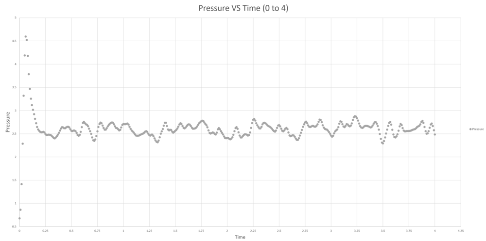
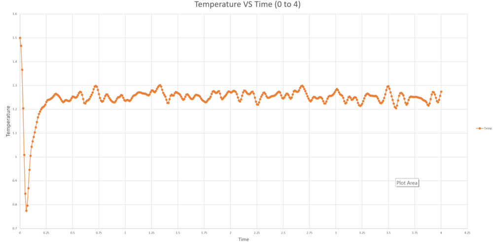
The energy, temperature and pressure plots for 0.001 timestep experiment were shown below. The simulation reached equilibrium at approximately 0.5 unit time.

Fig. 25 Total Energy VS Time Plot - Full Range	Fig.26 Pressure VS Time Plot - Full Range	Fig. Temperature VS Time Plot - Full Range
Fig. 27 Total Energy VS Time Plot - Enlarged	Fig. 28 Pressure VS Time Plot - Enlarged	Fig. Temperature VS Time Plot - Enlarged

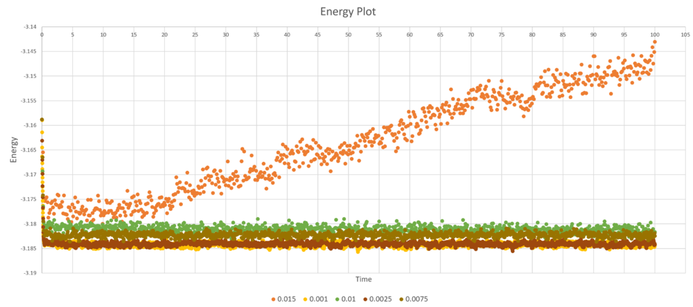
Below is the energy plot for all 5 different timmestep sizes, it is observed that 0.015 is a particularly bad timestep size and gives lattice with diverging energy. All other energy plots converges towards -3.185 reduced energy unit. 0.0025 timmestep size is the best balance timestep with very similar accuracy as 0.001 timestep, and shorter amount of simulation time than 0.001 timestep.

Fig. 29 Total Energy VS Time Plot for Different Timesteps

Running simulations under specific conditions

TASK: Choose 5 temperatures (above the critical temperature $T^{*}=1.5$), and two pressures (you can get a good idea of what a reasonable pressure is in Lennard-Jones units by looking at the average pressure of your simulations from the last section). This gives ten phase points — five temperatures at each pressure. Create 10 copies of npt.in, and modify each to run a simulation at one of your chosen $(p,T)$ points. You should be able to use the results of the previous section to choose a timestep. Submit these ten jobs to the HPC portal. While you wait for them to finish, you should read the next section.

5 temperatures chosen were $T^{*}=1.5,2.0,2.5,3.0and3.5$ at timesteps of 0.0025. For further invesstigation, simulations at other temperature points (i.e. 4.0, 4.5, 5.0, 5.5, 6.0, 6.5, 7.0, 8.0 amd 9.0) were performed.

TASK: We need to choose $\gamma$ so that the temperature is correct $T=\mathfrak{𝔗}$ if we multiply every velocity $\gamma$. We can write two equations: $\frac{1}{2}\sum _i{m}_i{v}_i^2=\frac{3}{2}N{k}_{B}T$ $\frac{1}{2}\sum _i{m}_i{\left(\gamma v_i\right)}^2=\frac{3}{2}N{k}_B\mathfrak{𝔗}$ Solve these to determine $\gamma$.

$\frac{1}{2}\sum _i{m}_i{\left(\gamma v_i\right)}^2=\frac{{\gamma }^2}{2}\sum _i{m}_i{v}_i^2$ $=\frac{3{\gamma }^2}{2}N{k}_{B}T=\frac{3}{2}N{k}_B\mathfrak{𝔗}$

$\therefore \gamma =(\frac{\mathfrak{𝔗}}{T}{)}^{\frac{1}{2}}$

TASK: Use the manual page to find out the importance of the three numbers 100 1000 100000. How often will values of the temperature, etc., be sampled for the average? How many measurements contribute to the average? Looking to the following line, how much time will you simulate?

The code:

 ave/time 100 1000 100000 

specify the number of input values and averages them every timestep. The first number (i.e. 100) is Nevery, which uses the input values every this many timesteps. The second value (i.e. 1000) is Nrepeat, which is the number of times to use input values for calculating averages. Finally, 100000 is the Nfreq value, which calculates averages every this many timesteps. So take our input file as an example, among 100000 repeats our simulation collected an averaging calculation is performed every 100000 data, which means one cycle of averaging is performed to the whole set of data, where every 100 data points will be taken to give an average value. Then final averaged quantity will be calculated from the 1000 averaged values.

TASK: When your simulations have finished, download the log files as before. At the end of the log file, LAMMPS will output the values and errors for the pressure, temperature, and density $\left(\frac{N}{V}\right)$. Use software of your choice to plot the density as a function of temperature for both of the pressures that you simulated. Your graph(s) should include error bars in both the x and y directions. You should also include a line corresponding to the density predicted by the ideal gas law at that pressure. Is your simulated density lower or higher? Justify this. Does the discrepancy increase or decrease with pressure?

Fig. 30 Density VS Temperature Plot

The above task was discussed in the lab report above, please refer to "Equation of State" section in Results and Discussion.

Calculating Heat Capacities Using Statistical Physics

TASK: As in the last section, you need to run simulations at ten phase points. In this section, we will be in density-temperature $({\rho }^{*},T^{*})$ phase space, rather than pressure-temperature phase space. The two densities required at 0.2 and 0.8, and the temperature range is $2.0,2.2,2.4,2.6,2.8$. Plot $C_V/V$ as a function of temperature, where $V$ is the volume of the simulation cell, for both of your densities (on the same graph). Is the trend the one you would expect? Attach an example of one of your input scripts to your report.

Figure. 31 Heat capacity per unit volume VS Temperature Plot at $\rho =0.2and0.8$

The above task was discussed in the lab report above, please refer to "Heat Capacity" section in Results and Discussion.

- DEFINE SIMULATION BOX GEOMETRY - variable density equal 0.2 lattice sc ${density} region box block 0 15 0 15 0 15 create_box 1 box create_atoms 1 box - DEFINE PHYSICAL PROPERTIES OF ATOMS - mass 1 1.0 pair_style lj/cut/opt 3.0 pair_coeff 1 1 1.0 1.0 neighbor 2.0 bin - SPECIFY THE REQUIRED THERMODYNAMIC STATE - variable T equal 2.0 variable timestep equal 0.0025 - ASSIGN ATOMIC VELOCITIES - velocity all create ${T} 12345 dist gaussian rot yes mom yes - SPECIFY ENSEMBLE - timestep ${timestep} fix nve all nve - THERMODYNAMIC OUTPUT CONTROL - thermo_style custom time etotal temp press thermo 10 - RECORD TRAJECTORY - dump traj all custom 1000 output-1 id x y z - RUN SIMULATION TO MELT CRYSTAL - run 10000 unfix nve reset_timestep 0 - BRING SYSTEM TO REQUIRED STATE - variable tdamp equal ${timestep}*100 fix nvt all nvt temp ${T} ${T} ${tdamp} run 10000 reset_timestep 0 - MEASURE SYSTEM STATE - unfix nvt fix nve all nve thermo_style custom atoms etotal temp vol variable temp equal temp variable temp2 equal temp*temp variable energy equal etotal variable volume equal vol variable energy2 equal etotal*etotal variable atoms equal atoms fix aves all ave/time 100 1000 100000 v_temp v_temp2 v_energy v_energy2 run 100000 variable avetemp equal f_aves[1] variable avetemp2 equal f_aves[2] variable aveenergy equal f_aves[3] variable aveenergy2 equal f_aves[4] variable heatcapacity equal ${atoms}*${atoms}*(${aveenergy2}-${aveenergy}*${aveenergy})/${avetemp2} print "Averages" print "--------" print "Heat Capacity: ${heatcapacity}" print "Volume: ${volume}"

Structural Properties and The Radial Distribution Function

TASK: perform simulations of the Lennard-Jones system in the three phases. When each is complete, download the trajectory and calculate g(r) and \int g(r)\mathrm{d}r. Plot the RDFs for the three systems on the same axes, and attach a copy to your report. Discuss qualitatively the differences between the three RDFs, and what this tells you about the structure of the system in each phase. In the solid case, illustrate which lattice sites the first three peaks correspond to. What is the lattice spacing? What is the coordination number for each of the first three peaks?

Questions are answered in "Radial Distribution Functions" section in Results and Discussion of the report above.

Figure. 32 Radial Distribution Function Plot

Figure. 33 $\int g(r)\mathrm{d}r$ Plot

Dynamimcal Properties and diffusion coefficient

Mean Squared Displacement

TASK: In the D subfolder, there is a file liq.in that will run a simulation at specified density and temperature to calculate the mean squared displacement and velocity autocorrelation function of your system. Run one of these simulations for a vapour, liquid, and solid. You have also been given some simulated data from much larger systems (approximately one million atoms). You will need these files later.

TASK: make a plot for each of your simulations (solid, liquid, and gas), showing the mean squared displacement (the "total" MSD) as a function of timestep. Are these as you would expect? Estimate D in each case. Be careful with the units! Repeat this procedure for the MSD data that you were given from the one million atom simulations.

Answers to questions in task was discussed in "Mean Squared Displacement and Diffusion Coefficient" section in Results and Discussion, please refer back to the report above.

Extension: Velocity Autocorrelation Function

TASK: In the theoretical section at the beginning, the equation for the evolution of the position of a 1D harmonic oscillator as a function of time was given. Using this, evaluate the normalised velocity autocorrelation function for a 1D harmonic oscillator (it is analytic!): $C\left(\tau \right)=\frac{\underset{-\mathrm{\infty }}{\overset{\mathrm{\infty }}{\int }}v\left(t\right)v(t+\tau )\mathrm{d}t}{\underset{-\mathrm{\infty }}{\overset{\mathrm{\infty }}{\int }}{v}^2\left(t\right)\mathrm{d}t}$ Be sure to show your working in your writeup. On the same graph, with x range 0 to 500, plot $C\left(\tau \right)$ with $\omega =1/2\pi$ and the VACFs from your liquid and solid simulations. What do the minima in the VACFs for the liquid and solid system represent? Discuss the origin of the differences between the liquid and solid VACFs. The harmonic oscillator VACF is very different to the Lennard Jones solid and liquid. Why is this? Attach a copy of your plot to your writeup.

TASK: Use the trapezium rule to approximate the integral under the velocity autocorrelation function for the solid, liquid, and gas, and use these values to estimate D in each case. You should make a plot of the running integral in each case. Are they as you expect? Repeat this procedure for the VACF data that you were given from the one million atom simulations. What do you think is the largest source of error in your estimates of D from the VACF?

For a 1D harmonic oscillator, $x(t)=A\cos (\omega t+\varphi )$ and $v(t)=-A\omega \sin (\omega t+\varphi )$. Substituting equation of $v(t)$ into the given equation of $C\left(\tau \right)$:

$C\left(\tau \right)=\frac{\underset{-\mathrm{\infty }}{\overset{\mathrm{\infty }}{\int }}-A\omega \sin (\omega t+\varphi )-A\omega \sin (\omega t+\varphi +\tau )\mathrm{d}t}{\underset{-\mathrm{\infty }}{\overset{\mathrm{\infty }}{\int }}-A\omega {\sin }^2(\omega t+\varphi )\mathrm{d}t}$

Using $\sin (\alpha +\beta )=\sin \alpha \cos \beta +\cos \alpha \sin \beta$:

$C\left(\tau \right)=\frac{\underset{-\mathrm{\infty }}{\overset{\mathrm{\infty }}{\int }}[{\sin }^2(\omega t+\varphi )\cos (\omega \tau )+\sin (\omega \tau )\sin (\omega t+\varphi )\cos (\omega t+\varphi )]\mathrm{d}t}{\underset{-\mathrm{\infty }}{\overset{\mathrm{\infty }}{\int }}{\sin }^2(\omega t+\varphi )\mathrm{d}t}$

$\because \sin (\omega t+\varphi )\cos (\omega t+\varphi )=0$

$C\left(\tau \right)=\frac{\underset{-\mathrm{\infty }}{\overset{\mathrm{\infty }}{\int }}{\sin }^2(\omega t+\varphi )\cos (\omega \tau )\mathrm{d}t}{\underset{-\mathrm{\infty }}{\overset{\mathrm{\infty }}{\int }}{\sin }^2(\omega t+\varphi )\mathrm{d}t}=\cos (\omega \tau )$

Plots and answers to the task are included in the Results and Discussion section of the lab rerport above, please refer back.