Rep:LS:01023138jw7815

Abstract

The abstract is often confused with a conclusion because we're not really taught how to write one. It's a section you write at the end and doesn't go into as much detail as the conclusion but you sum up the relevance of the research (intro), what you have done, what results do you have to show that you have done this and the ultimate conclusion.

This lab, not only should provide an interesting computational invetigation, but also we want to help you start to get into the practice of proper scientific writing before your projects this or next year. The lab itself to start with is pretty self-explanatory. Work through the exercises and think about what each of your result mean physically. We ask you to perform an individual investigation at the end - there isn't really a wrong answer! - try to think about your own experiment before asking others what they did. If you present something interesting in an engaging way, you will score highly. If anything is not clear here, please ask me in the lab or by email. Reports should be submitted to Blackboard by the end of the week.

Introduction

Your introduction paints a picture of the background of the research; what has been done by others and where is the niche for your work. How will your work benefit the community - maybe it's a new technique. You open up the niche so the subsequent discussion inserts your work into the existing community or (for high impact journals like Nature) creates a question and novel direction that can be picked up and worked on by other interested parties. In this lab, it would be good if you can demonstrate some of the importance of your results and impact it had on Science and society.

Methods

Reproducibility of data reinforces the high standards and quality expected for a piece of work in a peer reviewed journal. It also engenders the work with legitimacy. Your Methods section, just like in synthesis, should be short and sweet. Just like "5ml of DMSO was added", in computational you say "the tip4p/2005 forcefield was used". Unlike Synthesis, you are encouraged to explain your choice for each of the methods (a little more verbose than Synthesis!).

Questions

Results and Discussion is exactly what it says on the tin - most of you will be good at writing this section! Present a result using a method described and discuss what this result means and how your results show it.

Introduction to Molecular Dynamics Simulation

Velocity-Verlet Algorithm

Figure 1: Verlet blabla of sin(x) between 0 and $2\pi$

Figure 2: Verlet blabla of sin(x) between 0 and $2\pi$

Using the velocity-Verlet algorithm to model the behaviour of the classic harmonic oscillator (Figure 1), we see a good fit between the analytical data modelled by the harmonic oscillator and the velocity-Verlet solution (top graph). The error, given by the absolute difference between the analytical result and that modelled by the velocity-Verlet solution, shows a series of maximums of increasing amplitude (bottom graph). The positions of the maxima in the error function can be linearly represented by the Equation 1, and shown in Figure 1.

$$\begin{gathered} \mathbf{y}=0.00042155x\mathbf{x}-0.000073022 \\ (1) \end{gathered}$$

When the error is at a minimum value, it corresponds to a maximum energy value of 0.500, suggesting that the true energy value of the system is 0.500. In contrast, when the error is at a maximum, it corresponds to the minimum of the energy function - the exact value of the minimum will depend on the timestep used. When timestep is increased, the error maxima increase at a greater rate as compared to a lower timestep, resulting in a greater amplitude of fluctuation in the energy. This is illustrated in Figure 2, where a higher timestep of 0.2 results in greater fluctuation in energy. This vale is also is the maximum threshold to obtain an error in energy of less than 1%, where the energy (0.5) experiences a maximal fluctuation of 0.05.

It is important to monitor the total energy of a physical system when modelling its behaviour numerically because when a system has equilibrated, the total energy should remain constant, indicating that energy has been completely redistributed amongst the colliding particles in the system.

Atomic Forces

For a single Lennard-Jones interaction, $\varphi \left(r\right)=4ϵ(\frac{{\sigma }^{12}}{r^{12}}-\frac{{\sigma }^6}{r^6})$, when the potential energy, $\varphi$, is zero: $r_0$= $\sigma$, and force is at the regime where repulsion dominates.

The equilibrium separation, $r_{eq}$, occurs when the force is zero, i.e.

$\mathbf{F}=-\frac{\mathrm{d}U}{\mathrm{d}\mathbf{r}}=0$ $\frac{\mathrm{d}U}{\mathrm{d}\mathbf{r}}=-48ϵ{\sigma }^{12}(\frac{1}{r^{13}})+24ϵ{\sigma }^6(\frac{1}{r^7})=0$ $\frac{1}{r^7}=2{\sigma }^6(\frac{1}{r^{13}})$

(1/R7) = 2σ6(1/R13)

dU/dR = -48εσ12(1/R13) + 24εσ6(1/R7)

When $\sigma =ϵ=1.0$,

$\underset{2\sigma }{\overset{\mathrm{\infty }}{\int }}\varphi \left(r\right)\mathrm{d}r=0.020671$

$\underset{2.5\sigma }{\overset{\mathrm{\infty }}{\int }}\varphi \left(r\right)\mathrm{d}r=0.0068127$

$\underset{3\sigma }{\overset{\mathrm{\infty }}{\int }}\varphi \left(r\right)\mathrm{d}r=0.0027416$

Periodic Boundary Conditions

Under standard conditions, density of water = 1 g/cm³ (or g/ml) and molar mass of water = 18.01528 g/mol

m of 1 ml water = ρV = 1 g

n of 1ml water = m/M_r = 0.05550843506 mol

Number of water molecules = nN_A = 3.342796 x 10²²

 

For 10000 water molecules, n of water = n.o.m./N_A = 1.660539 x 10^-20 mol

m of water = nM_r = 2.991507 x 10^-19 g

V of water = m/ρ = 2.991507 x 10^-19 ml

Final atom position = (0.5, 0.5, 0.5) + 1*(0.7, 0.6, 0.2) = (1.2, 1.1,0.7)

After applying periodic boundary conditions = (0.2, 0.1, 0.7)

Reduced Units

r=r*σ

r = 3.2(0.34 x 10^-9) = 1.088 x 10^-9 m

 

ϕ(r_eq) = ε = k_BT x N_A

ε = (1.38065 x 10^-23 JK^-1)(120 K)(6.02214 x 10²³ mol^-1) = 997.73546 J mol^-1 = 0.997735 kJ mol^-1

 

T = T*ε/k_BN_A

T = 1.5(997.73546 J mol^-1)/(1.38065 x 10^-23 JK^-1)(6.02214 x 10²³ mol^-1) = 180 K

Equilibration

Creating a Simulation Box

In simulations, atoms which are generated by the random style may be highly overlapping, causing many interatomic potentials to be computed as large energies and forces which would blow atoms out of the simulation box, causing LAMMPS to return an error. This can be avoided by imposing a limit on the maximum distance an atom can movie in a single timestep by using the fix nve/limit command, this allows the system to equilibrate at the energy minimum. Alternatively, the positions of the atom can be pre-defined by a known lattice type before running the simulation.

Lattice Types

Figure 3: Different lattice types with different arrangement of atoms within each unit cell image from https://wps.prenhall.com/wps/media/objects/3082/3156196/blb1107/bl11fg33.jpg

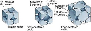
Different lattice types can be used to pre-define the position of atoms before a simulation. In these cubic lattice, the number density, $\rho =\frac{N}{V}$, where $N$ is the number of atoms per unit cell and the volume,$V=L^3$.

For example, in the simple cubic (sc), each unit cell contains $N=(\frac{1}{8})(8)=1$, if the number density, $\rho =0.8$: $L=\sqrt[3]{\frac{1}{0.8}}=1.07722$

When a box containing 1000 unit cells (and hence 1000 lattice points) is created, the create_atom function will generate 1000 atoms for the simulation, since each unit cell contains 1 atom

For a face-centered cubic (fcc), each unit cell contains $N=(\frac{1}{8})(8)+(\frac{1}{2})(6)=4$, if the number density, $\rho =1.2$: $L=\sqrt[3]{\frac{4}{1.2}}=1.49380$

When a box containing 1000 unit cells (and hence 1000 lattice points) is created, the create_atom function will generate 4000 atoms for the simulation, since each unit cell contains 4 atoms.

Properties of Atoms

After defining the position of the atoms, the properties were assigned using the following commands.

mass 1 1.0 
pair_style lj/cut 3.0
pair_coeff * * 1.0 1.0

mass 1 1.0: defines type 1 atoms as having a mass of 1.0

pair_style lj/cut 3.0: specifies a standard Lennard-Jones potential with no Coulomb between atom pairs, with global LJ cutoff set to distance $r=3.0$

pair_coeff * * 1.0 1.0: sets the pairwise forcefield coefficients for the symmetric I,J interaction to the same value of 1.0 for all (given by asterisk) type 1 with type 1 atom pairs

Choice of Algorithm

Since the ${\mathbf{x}}_i\left(0\right)$ and ${\mathbf{v}}_i\left(0\right)$ will be specified in this simulation, the velocity-Verlet algorithm will be used.

Running a Simulation

time step x number of timestep = total time. By defining the timestep and number of steps as a variable, we only need to change the timestep when running different simulations, and the number of steps will change correspondingly according to the formula. For the other formula, upon changing timestep, we have to manually calculate the number of steps and input them for each different simulation.

Checking Equilibration

Figure 4: Total Energy, Pressure, and Temperature against time when a timestep of 0.001 is used. Time is shown up to 1s to illustrate the point of equilibration.

Figure 5: Total Energy against time when a timestep of 0.001 is used

Figure 6: Comparison of Total Energy against time at different timesteps

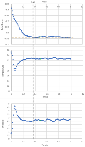
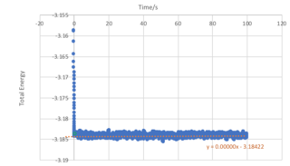
From Figure 5, we observe that an equilibrium energy value of -3.1482 is reached at a very early stage in the simulation with a timestep of 0.001. An expanded view showing the the first second of the simulation for the energy, temperature and pressure is shown in Figure 4, and it can be seen that equilibrium values are reached at approximately 0.38 seconds.

In simulations, shorter timesteps allow us to obtain more accurate calculations, although it can be costly and time-consuming to run such calculations. On the other hand, longer timesteps result in less accurate calculations. This balance is illustrated in Figure 6. When a long timestep of 0.015, the system stabilises at a minimum energy (at a value higher than the true vaue), but shortly after experiences a blowup as the errors start to propagate out of control, and therefore is a completely unacceptable timestep.

As the timestep decreases, an equilibrium is reached (0.01 and 0.0075), although it does not reach the true value of -3.184. Finally, as we further decrease the timestep to 0.0025, we see that a satisfactory value is obtained, which is identical to the most accurate value calculated at even lower timesteps. The balance in this simulation is thus to use a timestep of 0.0025, as it is high enough to avoid the high cost and time of simulations, yet low enough to obtain an acceptable calculation.

Running Simulations under Specific Conditions

Thermostats and Barostats

$\gamma =\sqrt{\frac{\mathfrak{𝔗}}{T}}$

Examining the Input Script

fix aves all ave/time 100 1000 100000 v_dens v_temp v_press v_dens2 v_temp2 v_press2

For the command ave/time, 100, 1000 and 100000 corresponds to Nevery, Nrepeat, and Nfreq respectively. These arguments specify on what timesteps the input values will be used in order to contribute to the average. Specifically, the final averaged quantities are generated on timesteps that are a multiple of Nfreq, and the average is over Nrepeat quantities, computed in the preceding portion of the simulation every Nevery timesteps.

Plotting the Equations of State

Figure 4: Total Energy, Pressure, and Temperature against time when a timestep of 0.001 is used. Time is shown up to 1s to illustrate the point of equilibration.

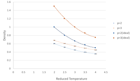
At both pressures, the simulated density (p=2 and p=3) is lower than the density as predicted by the ideal gas model. This is because the ideal gas model assumes that particles behave as point masses with no interactions, however, in the simulated model, the atoms are governed by Lennard-Jones interactions. At near interatomic separation in these simulations, the repulsion term dominates, and the atoms are pushed further apart from each other, resulting in a lower density. It is also noted that as temperature increases, the deviation from ideal behaviour is less in both cases. This is because at high temperatures, particles oscillate about the equilibrium to a greater extent and this fast oscillation makes the interaction between particles transient (as they have no time to react to these interactions). This is analogous to experiencing weaker interactions and hence tending towards ideal behaviour.

Comparing the simulations at higher and lower pressure, the one at higher pressure shows a greater deviation from ideality at all temperatures. This is a result of the greater interatomic interactions by atoms which are found closer together at high density.

Conclusion

Conclusions - tie up the research and what your results show. Reread your intro, what are you trying to do? How does your research do this?

References

Relevant supplementary material can be added at the end of the report so long as it supports your discussion. The marking criteria can be found in the Scheme for the Award of Honours (just like your bachelors and masters projects will be!) but importantly, work that presents an engaging dialogue and valid conclusion based on legitimate evidence will score highly. Presentation of results is arguably the most crucial part of science; you don't just show anything to the scientific community (for fear of inaccuracies being broadly spread and a retraction asked of you!), you show something relevant and defensible.